Predicting successful movies on IMDB
To help better assess which movies to bring into the Netflix streaming catalog, I have pulled data for the best and worst movies in the IMDB database and created two models from that data to predict ratings for other movies. A total of 350 records were downloaded: the top 250, and the bottom 100.
I collected data from both the IMDB website and the OMDB API, including columns for:
- Ratings from:
- IMDB
- Metacritic
- Rotten Tomatoes
- Number of IMDB user ratings
- Number of user reviews on IMDB
- Number of critic reviews on IMDB
- Gross revenue
- Actors
- Awards
- Country
- DVD release data
- Director
- Genre
- Languages
- Plot synopsis
- Producer
- Release date
- Running time
- Writer
- Year
Many of the columns (Plot and Actors, for example) were parsed for key word entries. I kept up to 50 terms from each key word search, and created new features recording the presence of those key words and the column it was found in (e.g. “director_sidney lumet” and “country_france”).
Feature Engineerings
v = CountVectorizer(
            binary= True,
            token_pattern= u'(?u)\w+.?\w?.? \w+',
            max_features=50
    )
data = v.fit_transform(X.Actors).todense()
names = v.get_feature_names()

temp_df = pd.DataFrame(data,columns=names)

for i in temp_df.columns:
    X.insert(len(X.columns)-1,"actor_"+i,temp_df[i].values)


v = CountVectorizer(
        binary= True,
        token_pattern= '(?u)\w+.?\w+',
        max_features=50
    )
data = v.fit_transform(X.Country).todense()
names = v.get_feature_names()

temp_df = pd.DataFrame(data,columns=names)

for i in temp_df.columns:
    X.insert(len(X.columns)-1,"country_"+i,temp_df[i].values)

v = CountVectorizer(
            binary= True,
            max_features=50
    )
data = v.fit_transform(X.Plot).todense()
names = v.get_feature_names()

temp_df = pd.DataFrame(data,columns=names)

for i in temp_df.columns:
    X.insert(len(X.columns)-1,"plot_"+i,temp_df[i].values)
Regression model
Performance
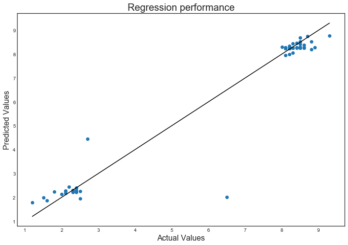
I first ran a random forest regressor on the data to create a predictive model for the IMDB rating based on the other data collected. The performance of the regressor can be seen in the figure below. The good and bad movie clusters are clearly visible, and largely predicted accurately. There are two points that were not fit well, however, indicating either the failure of the model, or the fickleness of the reviewers.
I ran a grid search over several parameters for a random forest model. The best model used 100 trees with 5 levels of depth and automatic feature selection. The R-squared performance metric for this is 0.9622 +/- 0.0244 across a cross validation of 3 KFolds, and 0.9496 on the holdout set (20% of the data).
plt.subplots(figsize=(12,8))
plt.scatter(y_test,randforest_pred)
plt.plot((min(y_test),max(y_test)),(min(y_test),max(y_test)), c='k')
plt.xlabel("Actual Values",fontsize=16)
plt.ylabel("Predicted Values",fontsize=16)
plt.title("Regression performance",fontsize=20)
plt.show()

Important features
Also shown in the results of the regression model are the relative importances of the features. The top five most important features in the model are shown in the table below. The number of ratings on IMDB is the strangest predictor in this set, followed by the ratings on other sites, the year of release, and the running time of the movie.
pd.DataFrame(zip(X_train.columns,randforest_gs.best_estimator_.steps[1][1].feature_importances_)\
                           ,columns=['feat','import']).sort_values('import',ascending=False).head()
| feat | import | |
|---|---|---|
| 3 | imdbVotes | 0.848560 |
| 4 | Rotten Tomatoes | 0.070706 |
| 0 | Metascore | 0.068943 |
| 2 | Year | 0.002933 |
| 1 | Runtime | 0.001881 |
Classification model
Of course the goal isn’t to rate the movies we consider, but rather to predict whether they are popular or not. To answer this question, I made a classification model with a random forest classifier. The fitting procedure is nearly identical. The same features were used, but I replaced the IMDB rating with a flag (1 for movies from the top movies list and 0 for the worst movies) as the target.
Performance
Accuracy becomes the metric for classification problems, and several items from my grid search achieved the highest average score, but the gs_best_predictor selected had higher variance, so the other models should also be explored.
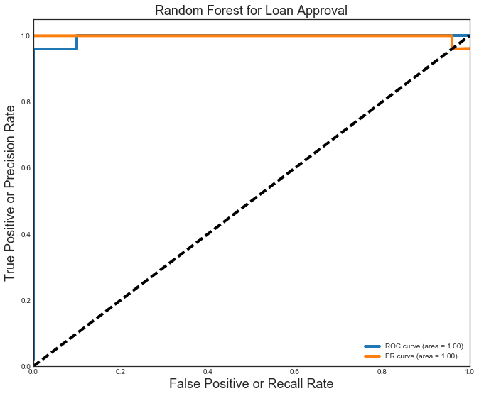
Regardless, I was able to achieve an accuracy of 0.97 on the test set, and the ROC and PR curve areas are both very high. The confusion matrix shows that only 2 of the 70 holdout movies were classified incorrectly.
rf_class_gs.score(X_test_class,y_test_class)
0.97142857142857142
print classification_report(y_test_class,rf_class_pred)
print ""
print pd.DataFrame(confusion_matrix(y_test_class,rf_class_pred,labels=[1,0]),\
                   columns=['pred_1','pred_0'],index=['is_1','is_0'])


# use the predicted probablitites to calculate AUC of ROC and PRCurve
Y_score = rf_class_gs.best_estimator_.predict_proba(X_test)[:,1]


# For class 1, find the area under the curve
FPR, TPR, _ = roc_curve(y_test_class, Y_score)
ROC_AUC = auc(FPR, TPR)

PREC, REC, _ = precision_recall_curve(y_test_class, Y_score)
PR_AUC = auc(REC, PREC)

# Plot of a ROC curve for class 1 (has_cancer)
plt.figure(figsize=[11,9])
plt.plot(FPR, TPR, label='ROC curve (area = %0.2f)' % ROC_AUC, linewidth=4)
plt.plot(REC, PREC, label='PR curve (area = %0.2f)' % PR_AUC, linewidth=4)
plt.plot([0, 1], [0, 1], 'k--', linewidth=4)
plt.xlim([0.0, 1.0])
plt.ylim([0.0, 1.05])
plt.xlabel('False Positive or Recall Rate', fontsize=18)
plt.ylabel('True Positive or Precision Rate', fontsize=18)
plt.title('Random Forest for Loan Approval', fontsize=18)
plt.legend(loc="lower right")
plt.show()
             precision    recall  f1-score   support

          0       1.00      0.90      0.95        20
          1       0.96      1.00      0.98        50

avg / total       0.97      0.97      0.97        70


      pred_1  pred_0
is_1      50       0
is_0       2      18

Feature importances
Several of the same features are important to the classifier as were important to the regressor. The number of IMDB votes in particular is still the most important feature. The number of reviews by critics and users are next, followed by the running time and then scores on other review sites. An interesting difference between the regressor and classifier is the reduced importance of outside ratings in making classification decisions.
print ""
print pd.DataFrame(zip(rf_class_gs.cv_results_['mean_test_score'],\
                 rf_class_gs.cv_results_['std_test_score']\
                ), columns=["score","score_err"]).sort_values("score",ascending=False).head()
print ""
rf_imps = pd.DataFrame(zip(X_train_class.columns,rf_class_gs.best_estimator_.steps[1][1].feature_importances_)\
                           ,columns=['feat','import'])

print rf_imps.sort_values('import',ascending=False).head(10)
       score  score_err
40  0.989247   0.008710
39  0.989247   0.008803
38  0.989247   0.008803
19  0.989247   0.008803
16  0.985663   0.013536

                    feat    import
3              imdbVotes  0.178194
7    NumberCriticReviews  0.156770
6      NumberUserReviews  0.124143
1                Runtime  0.092799
4        Rotten Tomatoes  0.061476
214          genre_drama  0.051764
0              Metascore  0.040188
5                  Gross  0.039270
219         genre_horror  0.028926
212         genre_comedy  0.019035
Next steps
First, there are several models that have very similar performance that I would like to explore further. I expect these other models to confirm the story seen in the two models presented here, or that there is another compelling message hidden in the data.
I am very interested in pulling more information from IMDB about the reviews submitted by users. In particular, I think that the proportion of users finding a review useful will become a strong information stream by which to judge users and reviews submitted for each movie. It may even be that several key user accounts can be identified as strategic markers on movie popularity… allowing for new movies to be classified before a critical mass of users have viewed and rated the movies on IMDB.