
Titanic survival predictions
I’ve put together a small analysis to demonstrate how we can create, tune, and evaluate models. I looked at the dataset of Titanic passengers and attempted to predict their survival outcomes based on information from the passenger list. I used a Logistic Regression, kNN, Decision Tree, and Random Forest model. The hyperparameters for each were tuned across a grid space that allowed for full computation in less than 5 minutes.
I am able to extract some information from the Names column which are included in the fit. Next steps are to determine which extracted features are important and start to limit them. The full roster from the training set is used in the model, but I expect some names are more important than others. I can limit the features output from my CountVectorizer to increase the efficiency of the model.
I also impute some ages, but they are not included in the model as I did not implement the fit in a manner to prevent information leaking from the test set into the training set.
I used a Train/Test split with 20% of the data held back to validate and compare the models. In tuning the hyperparameters for each model, I used KFolds validation with 5 folds.
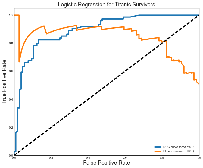
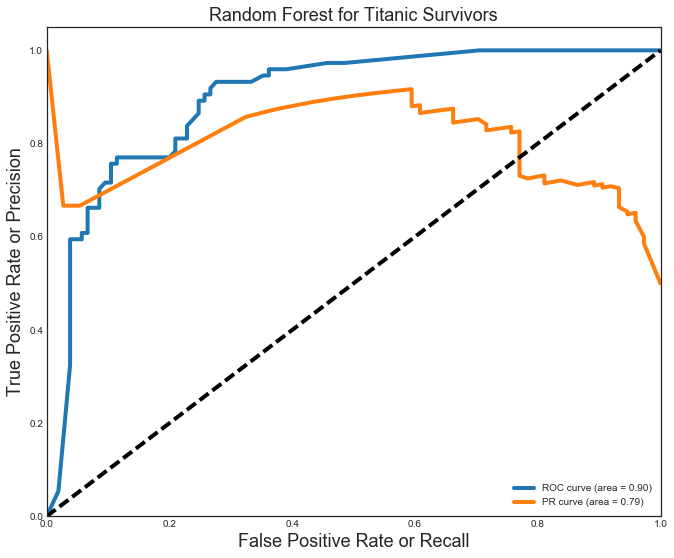
Comparing the models, I see that the Logistic Regression model fared the best with precision(P) and recall(R) at 0.85. The Random Forest was very close with P=R=0.84. Both these models fare well with an area under the curve (AUC) for the ROC = 0.90. The Logistic Regression model again differentiated itself with an AUC for the PR curve of 0.84 (beating the 0.79 for the Random Forest). The ROC (blue) and PR (orange) curves for the Random Forest model are shown below.
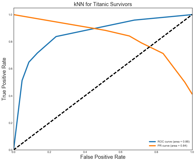
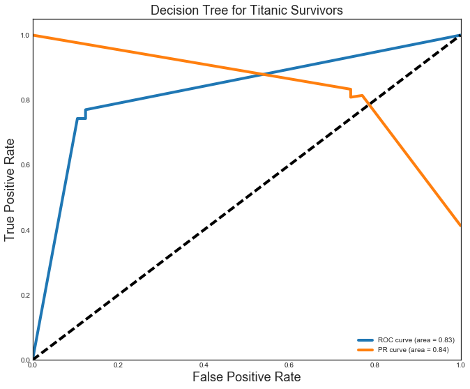
The kNN (P=R=0.8) and Decision Tree (P=R=0.83) models were close, but not quite as good as the others. They also vell behind in the AUC ROC (kNN=0.86,DT=0.83) and AUC PR curve (both=0.84).

The upshot of this analysis is that we are able to predict Titanic survival with over 80% accuracy using one of 4 models.
We have more information on the data stored in this database. The details can be found at Kaggle.
df = pd.read_csv("titanic_data.csv")
df.head()
| PassengerId | Survived | Pclass | Name | Sex | Age | SibSp | Parch | Ticket | Fare | Cabin | Embarked | |
|---|---|---|---|---|---|---|---|---|---|---|---|---|
| 0 | 1 | 0 | 3 | Braund, Mr. Owen Harris | male | 22.0 | 1 | 0 | A/5 21171 | 7.2500 | NaN | S |
| 1 | 2 | 1 | 1 | Cumings, Mrs. John Bradley (Florence Briggs Th... | female | 38.0 | 1 | 0 | PC 17599 | 71.2833 | C85 | C |
| 2 | 3 | 1 | 3 | Heikkinen, Miss. Laina | female | 26.0 | 0 | 0 | STON/O2. 3101282 | 7.9250 | NaN | S |
| 3 | 4 | 1 | 1 | Futrelle, Mrs. Jacques Heath (Lily May Peel) | female | 35.0 | 1 | 0 | 113803 | 53.1000 | C123 | S |
| 4 | 5 | 0 | 3 | Allen, Mr. William Henry | male | 35.0 | 0 | 0 | 373450 | 8.0500 | NaN | S |
df.info()
<class 'pandas.core.frame.DataFrame'>
RangeIndex: 891 entries, 0 to 890
Data columns (total 12 columns):
PassengerId    891 non-null int64
Survived       891 non-null int64
Pclass         891 non-null int64
Name           891 non-null object
Sex            891 non-null object
Age            714 non-null float64
SibSp          891 non-null int64
Parch          891 non-null int64
Ticket         891 non-null object
Fare           891 non-null float64
Cabin          204 non-null object
Embarked       889 non-null object
dtypes: float64(2), int64(5), object(5)
memory usage: 83.6+ KB
df[df.Age.isnull()].head()
| PassengerId | Survived | Pclass | Name | Sex | Age | SibSp | Parch | Ticket | Fare | Cabin | Embarked | |
|---|---|---|---|---|---|---|---|---|---|---|---|---|
| 5 | 6 | 0 | 3 | Moran, Mr. James | male | NaN | 0 | 0 | 330877 | 8.4583 | NaN | Q |
| 17 | 18 | 1 | 2 | Williams, Mr. Charles Eugene | male | NaN | 0 | 0 | 244373 | 13.0000 | NaN | S |
| 19 | 20 | 1 | 3 | Masselmani, Mrs. Fatima | female | NaN | 0 | 0 | 2649 | 7.2250 | NaN | C |
| 26 | 27 | 0 | 3 | Emir, Mr. Farred Chehab | male | NaN | 0 | 0 | 2631 | 7.2250 | NaN | C |
| 28 | 29 | 1 | 3 | O'Dwyer, Miss. Ellen "Nellie" | female | NaN | 0 | 0 | 330959 | 7.8792 | NaN | Q |
for i in df.columns:
    print df[i].value_counts().head(10)
891    1
293    1
304    1
303    1
302    1
301    1
300    1
299    1
298    1
297    1
Name: PassengerId, dtype: int64
0    549
1    342
Name: Survived, dtype: int64
3    491
1    216
2    184
Name: Pclass, dtype: int64
Graham, Mr. George Edward                              1
Elias, Mr. Tannous                                     1
Madill, Miss. Georgette Alexandra                      1
Cumings, Mrs. John Bradley (Florence Briggs Thayer)    1
Beane, Mrs. Edward (Ethel Clarke)                      1
Roebling, Mr. Washington Augustus II                   1
Moran, Mr. James                                       1
Padro y Manent, Mr. Julian                             1
Scanlan, Mr. James                                     1
Ali, Mr. William                                       1
Name: Name, dtype: int64
male      577
female    314
Name: Sex, dtype: int64
24.0    30
22.0    27
18.0    26
19.0    25
30.0    25
28.0    25
21.0    24
25.0    23
36.0    22
29.0    20
Name: Age, dtype: int64
0    608
1    209
2     28
4     18
3     16
8      7
5      5
Name: SibSp, dtype: int64
0    678
1    118
2     80
5      5
3      5
4      4
6      1
Name: Parch, dtype: int64
CA. 2343        7
347082          7
1601            7
347088          6
CA 2144         6
3101295         6
382652          5
S.O.C. 14879    5
PC 17757        4
4133            4
Name: Ticket, dtype: int64
8.0500     43
13.0000    42
7.8958     38
7.7500     34
26.0000    31
10.5000    24
7.9250     18
7.7750     16
26.5500    15
0.0000     15
Name: Fare, dtype: int64
C23 C25 C27        4
G6                 4
B96 B98            4
D                  3
C22 C26            3
E101               3
F2                 3
F33                3
B57 B59 B63 B66    2
C68                2
Name: Cabin, dtype: int64
S    644
C    168
Q     77
Name: Embarked, dtype: int64
Null value analysis
It seems most columns have no null values. The df.info() summary shows several columns already hold numerical data (for which the non-null value read out is accurate). Furthermore, the .value_counts() method on each series shows none of the typical null value entries (i.e. *,-,None,NA,999,-1,""). The upshot is only three columns are missing any data: Age, Cabin, and Embarked.
The Cabin column has relatively few values, and seems overly specific to be much help. I chose to drop it. The Embarked column is only missing 2 values, so there is not much pay off for the effort to re-integrate them. The Age coumn is missing 177 values which need to be imputed, and 15 more that are 0.0000 (though after research I see these VIPs like the ship designer). I will use a linear regression model on Pclass, Sex, Fare, Embarked, etc. to impute Age values that are missing.
df[df["Fare"] < 0.001].sort_values("Ticket")
# reasearching several of these individuals shows they were employees
# and much more likely to have died
# add a feature that is 1 for free_fare
| PassengerId | Survived | Pclass | Name | Sex | Age | SibSp | Parch | Ticket | Fare | Cabin | Embarked | |
|---|---|---|---|---|---|---|---|---|---|---|---|---|
| 806 | 807 | 0 | 1 | Andrews, Mr. Thomas Jr | male | 39.0 | 0 | 0 | 112050 | 0.0 | A36 | S |
| 633 | 634 | 0 | 1 | Parr, Mr. William Henry Marsh | male | NaN | 0 | 0 | 112052 | 0.0 | NaN | S |
| 815 | 816 | 0 | 1 | Fry, Mr. Richard | male | NaN | 0 | 0 | 112058 | 0.0 | B102 | S |
| 263 | 264 | 0 | 1 | Harrison, Mr. William | male | 40.0 | 0 | 0 | 112059 | 0.0 | B94 | S |
| 822 | 823 | 0 | 1 | Reuchlin, Jonkheer. John George | male | 38.0 | 0 | 0 | 19972 | 0.0 | NaN | S |
| 277 | 278 | 0 | 2 | Parkes, Mr. Francis "Frank" | male | NaN | 0 | 0 | 239853 | 0.0 | NaN | S |
| 413 | 414 | 0 | 2 | Cunningham, Mr. Alfred Fleming | male | NaN | 0 | 0 | 239853 | 0.0 | NaN | S |
| 466 | 467 | 0 | 2 | Campbell, Mr. William | male | NaN | 0 | 0 | 239853 | 0.0 | NaN | S |
| 481 | 482 | 0 | 2 | Frost, Mr. Anthony Wood "Archie" | male | NaN | 0 | 0 | 239854 | 0.0 | NaN | S |
| 732 | 733 | 0 | 2 | Knight, Mr. Robert J | male | NaN | 0 | 0 | 239855 | 0.0 | NaN | S |
| 674 | 675 | 0 | 2 | Watson, Mr. Ennis Hastings | male | NaN | 0 | 0 | 239856 | 0.0 | NaN | S |
| 179 | 180 | 0 | 3 | Leonard, Mr. Lionel | male | 36.0 | 0 | 0 | LINE | 0.0 | NaN | S |
| 271 | 272 | 1 | 3 | Tornquist, Mr. William Henry | male | 25.0 | 0 | 0 | LINE | 0.0 | NaN | S |
| 302 | 303 | 0 | 3 | Johnson, Mr. William Cahoone Jr | male | 19.0 | 0 | 0 | LINE | 0.0 | NaN | S |
| 597 | 598 | 0 | 3 | Johnson, Mr. Alfred | male | 49.0 | 0 | 0 | LINE | 0.0 | NaN | S |
df = df.drop("Cabin", axis=1)
df = df.drop("Ticket", axis=1)
df = df.drop("PassengerId", axis=1)
print df[df["Embarked"].isnull()]
df.Embarked.fillna("S",inplace=True)
# https://www.encyclopedia-titanica.org/titanic-survivor/amelia-icard.html
# research shows these should both be set to S for Southampton
     Survived  Pclass                                       Name     Sex  \
61          1       1                        Icard, Miss. Amelie  female
829         1       1  Stone, Mrs. George Nelson (Martha Evelyn)  female

      Age  SibSp  Parch  Fare Embarked
61   38.0      0      0  80.0      NaN
829  62.0      0      0  80.0      NaN
df = pd.get_dummies(df,columns=["Pclass","Sex","Embarked"],drop_first=True)
df['free_fare'] = df.Fare.map(lambda x: 1 if x < 0.001 else 0)
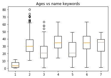
The Age of a person is related to some key words in the Name column
master = df[["Master." in x for x in df["Name"]]]["Age"].dropna()
rev = df[["Rev." in x for x in df["Name"]]]["Age"].dropna()
mr = df[["Mr." in x for x in df["Name"]]]["Age"].dropna()
miss = df[["Miss." in x for x in df["Name"]]]["Age"].dropna()
mrs = df[["Mrs." in x for x in df["Name"]]]["Age"].dropna()
quot = df[['"' in x for x in df["Name"]]]["Age"].dropna()
paren = df[["(" in x for x in df["Name"]]]["Age"].dropna()
both = df[["(" in x and '"' in x for x in df["Name"]]]["Age"].dropna()
plt.boxplot([master.values,mr.values,miss.values, \
             mrs.values,quot.values,paren.values, \
             both.values])
plt.title("Ages vs name keywords")
plt.show()
df["has_master"] = df.Name.map(lambda x: 1 if 'Master.' in x else 0)
df["has_rev"] = df.Name.map(lambda x: 1 if 'Rev.' in x else 0)
df["has_mr"] = df.Name.map(lambda x: 1 if 'Mr.' in x else 0)
df["has_miss"] = df.Name.map(lambda x: 1 if 'Miss.' in x else 0)
df["has_mrs"] = df.Name.map(lambda x: 1 if 'Mrs.' in x else 0)
df["has_quote"] = df.Name.map(lambda x: 1 if '"' in x else 0)
df["has_parens"] = df.Name.map(lambda x: 1 if '(' in x else 0)
df["last_name"] = df.Name.map(lambda x: x.replace(",","").split()[0] )
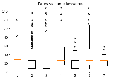
Note that those name columns also have a bearing on the fare.
master = df[["Master." in x for x in df["Name"]]]["Fare"].dropna()
rev = df[["Rev." in x for x in df["Name"]]]["Fare"].dropna()
mr = df[["Mr." in x for x in df["Name"]]]["Fare"].dropna()
miss = df[["Miss." in x for x in df["Name"]]]["Fare"].dropna()
mrs = df[["Mrs." in x for x in df["Name"]]]["Fare"].dropna()
quot = df[['"' in x for x in df["Name"]]]["Fare"].dropna()
paren = df[["(" in x for x in df["Name"]]]["Fare"].dropna()
both = df[["(" in x and '"' in x for x in df["Name"]]]["Fare"].dropna()
plt.boxplot([master.values,mr.values,miss.values, \
             mrs.values,quot.values,paren.values,both.values])
plt.title("Fares vs name keywords")
plt.ylim(0,150)
plt.show()
# master
Impute the age….
dropping for now, will finish when I have more time
X = df.iloc[:,2:]
y = df.iloc[:,0]
from sklearn.preprocessing import StandardScaler, MaxAbsScaler, MinMaxScaler, Imputer
from sklearn.preprocessing import OneHotEncoder, LabelEncoder, LabelBinarizer
from sklearn.base import TransformerMixin, BaseEstimator
from sklearn.model_selection import StratifiedKFold, cross_val_score, GridSearchCV
from sklearn.pipeline import make_pipeline, Pipeline, FeatureUnion
from sklearn.linear_model import LogisticRegressionCV, ElasticNetCV
from sklearn.neighbors import KNeighborsClassifier, KNeighborsRegressor
from sklearn.metrics import classification_report, confusion_matrix, accuracy_score
from sklearn.feature_extraction.text import CountVectorizer
from sklearn import tree
X.head()
| Age | SibSp | Parch | Fare | Pclass_2 | Pclass_3 | Sex_male | Embarked_Q | Embarked_S | free_fare | has_quote | has_parens | last_name | has_master | has_rev | has_mr | has_miss | has_mrs | |
|---|---|---|---|---|---|---|---|---|---|---|---|---|---|---|---|---|---|---|
| 0 | 22.0 | 1 | 0 | 7.2500 | 0 | 1 | 1 | 0 | 1 | 0 | 0 | 0 | Braund | 0 | 0 | 1 | 0 | 0 |
| 1 | 38.0 | 1 | 0 | 71.2833 | 0 | 0 | 0 | 0 | 0 | 0 | 0 | 1 | Cumings | 0 | 0 | 0 | 0 | 1 |
| 2 | 26.0 | 0 | 0 | 7.9250 | 0 | 1 | 0 | 0 | 1 | 0 | 0 | 0 | Heikkinen | 0 | 0 | 0 | 1 | 0 |
| 3 | 35.0 | 1 | 0 | 53.1000 | 0 | 0 | 0 | 0 | 1 | 0 | 0 | 1 | Futrelle | 0 | 0 | 0 | 0 | 1 |
| 4 | 35.0 | 0 | 0 | 8.0500 | 0 | 1 | 1 | 0 | 1 | 0 | 0 | 0 | Allen | 0 | 0 | 1 | 0 | 0 |
cols = [x for x in X.columns if x !='last_name' and x != 'Age']
u = StandardScaler()
v = ElasticNetCV()
g = GridSearchCV(Pipeline([('scale',u),('fit',v)]),{'fit__l1_ratio':(0.00001,0.1,0.2,0.3,0.4,0.5,0.6,0.7,0.8,0.9,1)})
g.fit(X[X.Age.notnull()].ix[:,cols],X.Age[X.Age.notnull()])
GridSearchCV(cv=None, error_score='raise',
       estimator=Pipeline(steps=[('scale', StandardScaler(copy=True, with_mean=True, with_std=True)), ('fit', ElasticNetCV(alphas=None, copy_X=True, cv=None, eps=0.001, fit_intercept=True,
       l1_ratio=0.5, max_iter=1000, n_alphas=100, n_jobs=1,
       normalize=False, positive=False, precompute='auto',
       random_state=None, selection='cyclic', tol=0.0001, verbose=0))]),
       fit_params={}, iid=True, n_jobs=1,
       param_grid={'fit__l1_ratio': (1e-05, 0.1, 0.2, 0.3, 0.4, 0.5, 0.6, 0.7, 0.8, 0.9, 1)},
       pre_dispatch='2*n_jobs', refit=True, return_train_score=True,
       scoring=None, verbose=0)
g.best_estimator_
Pipeline(steps=[('scale', StandardScaler(copy=True, with_mean=True, with_std=True)), ('fit', ElasticNetCV(alphas=None, copy_X=True, cv=None, eps=0.001, fit_intercept=True,
       l1_ratio=0.2, max_iter=1000, n_alphas=100, n_jobs=1,
       normalize=False, positive=False, precompute='auto',
       random_state=None, selection='cyclic', tol=0.0001, verbose=0))])
pd.DataFrame(g.cv_results_).sort_values("rank_test_score")
| mean_fit_time | mean_score_time | mean_test_score | mean_train_score | param_fit__l1_ratio | params | rank_test_score | split0_test_score | split0_train_score | split1_test_score | split1_train_score | split2_test_score | split2_train_score | std_fit_time | std_score_time | std_test_score | std_train_score | |
|---|---|---|---|---|---|---|---|---|---|---|---|---|---|---|---|---|---|
| 2 | 0.046002 | 0.000550 | 0.391722 | 0.429859 | 0.2 | {u'fit__l1_ratio': 0.2} | 1 | 0.413091 | 0.422948 | 0.366310 | 0.446579 | 0.395766 | 0.420050 | 0.002945 | 4.856305e-06 | 0.019311 | 0.011882 |
| 3 | 0.042412 | 0.000610 | 0.391685 | 0.430925 | 0.3 | {u'fit__l1_ratio': 0.3} | 2 | 0.412379 | 0.424478 | 0.366585 | 0.448172 | 0.396090 | 0.420125 | 0.000749 | 7.684356e-05 | 0.018953 | 0.012324 |
| 4 | 0.050115 | 0.000556 | 0.391633 | 0.431215 | 0.4 | {u'fit__l1_ratio': 0.4} | 3 | 0.412232 | 0.424710 | 0.366492 | 0.449001 | 0.396175 | 0.419933 | 0.005820 | 1.209189e-05 | 0.018948 | 0.012727 |
| 10 | 0.052624 | 0.000580 | 0.391569 | 0.430489 | 1 | {u'fit__l1_ratio': 1} | 4 | 0.412814 | 0.423898 | 0.365593 | 0.450084 | 0.396301 | 0.417486 | 0.004806 | 2.035405e-05 | 0.019566 | 0.014100 |
| 6 | 0.044164 | 0.000552 | 0.391485 | 0.431206 | 0.6 | {u'fit__l1_ratio': 0.6} | 5 | 0.412507 | 0.424419 | 0.365893 | 0.449813 | 0.396054 | 0.419386 | 0.000968 | 4.112672e-06 | 0.019303 | 0.013316 |
| 5 | 0.043362 | 0.000547 | 0.391462 | 0.431158 | 0.5 | {u'fit__l1_ratio': 0.5} | 6 | 0.412284 | 0.424680 | 0.366234 | 0.449498 | 0.395867 | 0.419297 | 0.000841 | 4.052337e-07 | 0.019056 | 0.013153 |
| 7 | 0.045165 | 0.000662 | 0.391385 | 0.430981 | 0.7 | {u'fit__l1_ratio': 0.7} | 7 | 0.412651 | 0.424263 | 0.365791 | 0.449899 | 0.395712 | 0.418780 | 0.000889 | 1.501678e-04 | 0.019373 | 0.013563 |
| 9 | 0.050791 | 0.000570 | 0.391225 | 0.430514 | 0.9 | {u'fit__l1_ratio': 0.9} | 8 | 0.412857 | 0.423943 | 0.365807 | 0.449975 | 0.395013 | 0.417623 | 0.004066 | 2.837103e-05 | 0.019394 | 0.014001 |
| 8 | 0.046530 | 0.000582 | 0.391185 | 0.430643 | 0.8 | {u'fit__l1_ratio': 0.8} | 9 | 0.412813 | 0.424076 | 0.365768 | 0.449945 | 0.394972 | 0.417907 | 0.001666 | 4.249577e-05 | 0.019392 | 0.013879 |
| 1 | 0.040549 | 0.000563 | 0.391117 | 0.426731 | 0.1 | {u'fit__l1_ratio': 0.1} | 10 | 0.413325 | 0.418232 | 0.364558 | 0.441993 | 0.395468 | 0.419967 | 0.001385 | 2.537861e-05 | 0.020145 | 0.010815 |
| 0 | 0.054007 | 0.000892 | -0.002510 | 0.002103 | 1e-05 | {u'fit__l1_ratio': 1e-05} | 11 | -0.002335 | 0.001980 | -0.006706 | 0.002114 | 0.001509 | 0.002216 | 0.012009 | 3.612715e-04 | 0.003356 | 0.000096 |
g.predict(X[X.Age.notnull()].ix[:,cols]).shape
(714,)
X.Age[X.Age.notnull()].shape
(714,)
g.score(X[X.Age.notnull()].ix[:,cols],X.Age[X.Age.notnull()])
0.42502999520596807
plt.scatter(X.Age[X.Age.notnull()],g.predict(X[X.Age.notnull()].ix[:,cols]))
plt.plot(X.Age[X.Age.notnull()],X.Age[X.Age.notnull()])
[<matplotlib.lines.Line2D at 0x141d71a90>]
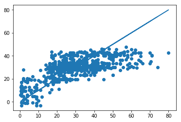
g.predict(X[X.Age.isnull()].ix[:,cols])
array([ 33.52360534,  33.89086473,  31.06711941,  28.61787182,
        21.53509477,  29.89157263,  40.0343745 ,  23.17295561,
        28.6178183 ,  28.60932366,  29.88960763,  31.36828054,
        23.17295561,  24.30249704,  42.3477308 ,  41.164614  ,
         5.36742999,  29.89157263,  29.88960763,  23.17247774,
        29.88960763,  29.88960763,  28.25535822,  29.89311202,
        20.8983758 ,  29.88960763,  33.53263137,  15.64632392,
        30.2580401 ,  29.89900576,  29.88180239,  -8.8549017 ,
        44.19505112,  42.46974728,   2.38825012,   1.51462849,
        32.58249212,  42.16295389,  32.18131372,  33.53263137,
        21.5367412 ,  11.87430425,  31.46704062,  29.89157263,
        12.75778031,  19.53630348,  16.10048191,  19.37239037,
        29.89980221,  42.95785004,  33.53263137,  23.17295561,
        42.40507536,  21.5367412 ,  32.42031237,  42.46879154,
        41.164614  ,  42.41144698,  21.5367412 ,  29.20392972,
        27.17867284,  28.25339321,  29.74517895,  11.87430425,
        18.84425395,  41.48063911,  29.89157263,  30.17068142,
        42.35410242,  28.61787182,  23.17130919,  21.53509477,
        31.36828054,  31.06706589,  23.17295561,  40.85440168,
        29.89157263,  33.53289643,  12.75778031,  29.89157263,
        33.54399452,  34.05652678,  32.33885522,  28.60932366,
        29.89980221,  33.53263137,  30.17068142,  29.88881117,
        27.67215956,  29.88960763,  42.52287645,  33.53263137,
        29.88960763,  34.05652678,  33.53294995,  29.89980221,
        42.13746742,  32.42031237,  12.75778031,  27.67215956,
        28.52569618,  29.79976782,  23.17449499,  40.82556834,
        29.88960763,  33.32364232,  28.61787182,  28.6178183 ,
        39.97393115,  28.6178183 ,  30.16740384,  29.80741376,
        32.59762471,  33.53162211,  38.6184621 ,  33.53263137,
        29.88960763,  19.52993187,  28.6178183 ,  23.17295561,
        28.90935301,  28.59891626,  29.88960763,  22.46608724,
        23.27632426,  28.61787182,  29.89157263,  42.25980248,
        29.90235086,  21.00860478,  33.53263137,  33.53284418,
        42.80011565,  27.72143383,  29.2722514 ,  29.89597924,
        29.89157263,  21.53573193,  29.89157263,  29.89311202,
        42.52112426,  34.05652678,  23.16801761,  29.2722514 ,
        21.53695401,   3.73121558,  42.46178276,  33.4338713 ,
        23.1731149 ,  34.05652678,  29.89157263,  29.89157263,
        42.41781859,  29.80741376,  41.01323456,  31.25805156,
        28.61787182,  33.53263137,  33.53279066,  26.92090268,
        31.89641696,   1.51462849,  41.12670288,  42.80011565,
        33.54282596,  29.2722514 ,  33.53263137,  28.6178183 ,
        29.88960763,  41.13939259,  11.87430425,  40.76604774,
        28.6178183 ,  -0.12158593,  29.87112993,  29.89157263,  14.9250125 ])
Aborted imputation
Drop rows not required
df = df.drop("Age",axis=1)
df = df.drop("Name",axis=1)
df.head()
| Survived | SibSp | Parch | Fare | Pclass_2 | Pclass_3 | Sex_male | Embarked_Q | Embarked_S | free_fare | has_master | has_rev | has_mr | has_miss | has_mrs | has_quote | has_parens | last_name | |
|---|---|---|---|---|---|---|---|---|---|---|---|---|---|---|---|---|---|---|
| 0 | 0 | 1 | 0 | 7.2500 | 0 | 1 | 1 | 0 | 1 | 0 | 0 | 0 | 1 | 0 | 0 | 0 | 0 | Braund |
| 1 | 1 | 1 | 0 | 71.2833 | 0 | 0 | 0 | 0 | 0 | 0 | 0 | 0 | 0 | 0 | 1 | 0 | 1 | Cumings |
| 2 | 1 | 0 | 0 | 7.9250 | 0 | 1 | 0 | 0 | 1 | 0 | 0 | 0 | 0 | 1 | 0 | 0 | 0 | Heikkinen |
| 3 | 1 | 1 | 0 | 53.1000 | 0 | 0 | 0 | 0 | 1 | 0 | 0 | 0 | 0 | 0 | 1 | 0 | 1 | Futrelle |
| 4 | 0 | 0 | 0 | 8.0500 | 0 | 1 | 1 | 0 | 1 | 0 | 0 | 0 | 1 | 0 | 0 | 0 | 0 | Allen |
X = df.iloc[:,1:]
y = df.iloc[:,0]
Make a Train/test split
from sklearn.model_selection import train_test_split
X_train, X_test, y_train, y_test, = train_test_split(X, y, test_size=0.2, random_state=42)
Define functions for grid search
class ModelTransformer(BaseEstimator,TransformerMixin):

    def __init__(self, model=None):
        self.model = model

    def fit(self, *args, **kwargs):
        self.model.fit(*args, **kwargs)
        return self

    def transform(self, X, **transform_params):
        return self.model.transform(X)

class SampleExtractor(BaseEstimator, TransformerMixin):
    """Takes in varaible names as a **list**"""

    def __init__(self, vars):
        self.vars = vars  # e.g. pass in a column names to extract

    def transform(self, X, y=None):
        if len(self.vars) > 1:
            return pd.DataFrame(X[self.vars]) # where the actual feature extraction happens
        else:
            return pd.Series(X[self.vars[0]])

    def fit(self, X, y=None):
        return self  # generally does nothing


class DenseTransformer(BaseEstimator,TransformerMixin):

    def transform(self, X, y=None, **fit_params):
#         print X.todense()
        return X.todense()

    def fit_transform(self, X, y=None, **fit_params):
        self.fit(X, y, **fit_params)
        return self.transform(X)

    def fit(self, X, y=None, **fit_params):
        return self
Logistic Regression
kf_shuffle = StratifiedKFold(n_splits=5,shuffle=True,random_state=777)

cols = [x for x in X.columns if x !='last_name']

pipeline = Pipeline([
    ('features', FeatureUnion([
        ('names', Pipeline([
                      ('text',SampleExtractor(['last_name'])),
                      ('dummify', CountVectorizer(binary=True)),
                      ('densify', DenseTransformer()),
                     ])),
        ('cont_features', Pipeline([
                      ('continuous', SampleExtractor(cols)),
                      ])),
        ])),
        ('scale', ModelTransformer()),
        ('fit', LogisticRegressionCV(solver='liblinear')),
])


parameters = {
    'scale__model': (StandardScaler(),MinMaxScaler()),
    'fit__penalty': ('l1','l2'),
    'fit__class_weight':('balanced',None),
    'fit__Cs': (5,10,15),
}

logreg_gs = GridSearchCV(pipeline, parameters, verbose=False, cv=kf_shuffle, n_jobs=-1)
print("Performing grid search...")
print("pipeline:", [name for name, _ in pipeline.steps])
print("parameters:")
print(parameters)


logreg_gs.fit(X_train, y_train)

print("Best score: %0.3f" % logreg_gs.best_score_)
print("Best parameters set:")
best_parameters = logreg_gs.best_estimator_.get_params()
for param_name in sorted(parameters.keys()):
    print("\t%s: %r" % (param_name, best_parameters[param_name]))
Performing grid search...
('pipeline:', ['features', 'scale', 'fit'])
parameters:
{'fit__class_weight': ('balanced', None), 'scale__model': (StandardScaler(copy=True, with_mean=True, with_std=True), MinMaxScaler(copy=True, feature_range=(0, 1))), 'fit__Cs': (5, 10, 15), 'fit__penalty': ('l1', 'l2')}
Best score: 0.837
Best parameters set:
	fit__Cs: 10
	fit__class_weight: None
	fit__penalty: 'l1'
	scale__model: StandardScaler(copy=True, with_mean=True, with_std=True)
cv_pred = pd.Series(logreg_gs.predict(X_test))
pd.DataFrame(zip(logreg_gs.cv_results_['mean_test_score'],\
                 logreg_gs.cv_results_['std_test_score']\
                )).sort_values(0,ascending=False).head(10)
| 0 | 1 | |
|---|---|---|
| 12 | 0.837079 | 0.030212 |
| 4 | 0.835674 | 0.035058 |
| 23 | 0.835674 | 0.034204 |
| 15 | 0.834270 | 0.031169 |
| 20 | 0.834270 | 0.033009 |
| 21 | 0.832865 | 0.037548 |
| 17 | 0.832865 | 0.033389 |
| 13 | 0.831461 | 0.035749 |
| 16 | 0.830056 | 0.034090 |
| 3 | 0.830056 | 0.038983 |
# logreg_gs.best_estimator_
confusion_matrix(y_test,cv_pred)
array([[94, 11],
       [16, 58]])
print classification_report(y_test,cv_pred)
             precision    recall  f1-score   support

          0       0.85      0.90      0.87       105
          1       0.84      0.78      0.81        74

avg / total       0.85      0.85      0.85       179
from sklearn.metrics import roc_curve, auc
plt.style.use('seaborn-white')

# Y_score = logreg_gs.best_estimator_.decision_function(X_test)
Y_score = logreg_gs.best_estimator_.predict_proba(X_test)[:,1]

# For class 1, find the area under the curve
FPR, TPR, _ = roc_curve(y_test, Y_score)
ROC_AUC = auc(FPR, TPR)
PREC, REC, _ = precision_recall_curve(y_test, Y_score)
PR_AUC = auc(REC, PREC)

# Plot of a ROC curve for class 1 (has_cancer)
plt.figure(figsize=[11,9])
plt.plot(FPR, TPR, label='ROC curve (area = %0.2f)' % ROC_AUC, linewidth=4)
plt.plot(REC, PREC, label='PR curve (area = %0.2f)' % PR_AUC, linewidth=4)
plt.plot([0, 1], [0, 1], 'k--', linewidth=4)
plt.xlim([0.0, 1.0])
plt.ylim([0.0, 1.05])
plt.xlabel('False Positive Rate', fontsize=18)
plt.ylabel('True Positive Rate', fontsize=18)
plt.title('Logistic Regression for Titanic Survivors', fontsize=18)
plt.legend(loc="lower right")
plt.show()
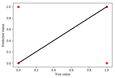
plt.scatter(y_test,cv_pred,color='r')
plt.plot(y_test,y_test,color='k')
plt.xlabel("True value")
plt.ylabel("Predicted Value")
plt.show()
kNN
kf_shuffle = StratifiedKFold(n_splits=5,shuffle=True,random_state=777)

cols = [x for x in X.columns if x !='last_name']

pipeline = Pipeline([
    ('features', FeatureUnion([
        ('names', Pipeline([
                      ('text',SampleExtractor(['last_name'])),
                      ('dummify', CountVectorizer(binary=True)),
                      ('densify', DenseTransformer()),
                     ])),
        ('cont_features', Pipeline([
                      ('continuous', SampleExtractor(cols)),
                      ])),
        ])),
        ('scale', ModelTransformer()),
        ('fit', KNeighborsClassifier()),
])


parameters = {
    'scale__model': (StandardScaler(),MinMaxScaler()),
    'fit__n_neighbors': (2,3,5,7,9,11,16,20),
    'fit__weights': ('uniform','distance'),
}

knn_gs = GridSearchCV(pipeline, parameters, verbose=False, cv=kf_shuffle, n_jobs=-1)
print("Performing grid search...")
print("pipeline:", [name for name, _ in pipeline.steps])
print("parameters:")
print(parameters)


knn_gs.fit(X_train, y_train)

print("Best score: %0.3f" % knn_gs.best_score_)
print("Best parameters set:")
best_parameters = knn_gs.best_estimator_.get_params()
for param_name in sorted(parameters.keys()):
    print("\t%s: %r" % (param_name, best_parameters[param_name]))
Performing grid search...
('pipeline:', ['features', 'scale', 'fit'])
parameters:
{'fit__n_neighbors': (2, 3, 5, 7, 9, 11, 16, 20), 'scale__model': (StandardScaler(copy=True, with_mean=True, with_std=True), MinMaxScaler(copy=True, feature_range=(0, 1))), 'fit__weights': ('uniform', 'distance')}
Best score: 0.829
Best parameters set:
	fit__n_neighbors: 5
	fit__weights: 'uniform'
	scale__model: MinMaxScaler(copy=True, feature_range=(0, 1))
cv_pred = pd.Series(knn_gs.predict(X_test))
pd.DataFrame(zip(knn_gs.cv_results_['mean_test_score'],\
                 knn_gs.cv_results_['std_test_score']\
                )).sort_values(0,ascending=False).head(10)
| 0 | 1 | |
|---|---|---|
| 9 | 0.828652 | 0.027271 |
| 11 | 0.827247 | 0.024505 |
| 5 | 0.821629 | 0.023673 |
| 25 | 0.818820 | 0.035553 |
| 7 | 0.818820 | 0.021308 |
| 31 | 0.816011 | 0.032000 |
| 27 | 0.814607 | 0.032273 |
| 29 | 0.811798 | 0.033521 |
| 19 | 0.810393 | 0.031341 |
| 17 | 0.810393 | 0.033816 |
# knn_gs.best_estimator_
confusion_matrix(y_test,cv_pred)
array([[91, 14],
       [21, 53]])
print classification_report(y_test,cv_pred)
             precision    recall  f1-score   support

          0       0.81      0.87      0.84       105
          1       0.79      0.72      0.75        74

avg / total       0.80      0.80      0.80       179
from sklearn.metrics import roc_curve, auc
plt.style.use('seaborn-white')

# Y_score = knn_gs.best_estimator_.decision_function(X_test)
Y_score = knn_gs.best_estimator_.predict_proba(X_test)[:,1]


# For class 1, find the area under the curve
FPR, TPR, _ = roc_curve(y_test, Y_score)
ROC_AUC = auc(FPR, TPR)

PREC, REC, _ = precision_recall_curve(y_test, Y_score)
PR_AUC = auc(REC, PREC)

# Plot of a ROC curve for class 1 (has_cancer)
plt.figure(figsize=[11,9])
plt.plot(FPR, TPR, label='ROC curve (area = %0.2f)' % ROC_AUC, linewidth=4)
plt.plot(REC, PREC, label='PR curve (area = %0.2f)' % PR_AUC, linewidth=4)
plt.plot([0, 1], [0, 1], 'k--', linewidth=4)
plt.xlim([0.0, 1.0])
plt.ylim([0.0, 1.05])
plt.xlabel('False Positive Rate', fontsize=18)
plt.ylabel('True Positive Rate', fontsize=18)
plt.title('kNN for Titanic Survivors', fontsize=18)
plt.legend(loc="lower right")
plt.show()
Decision Tree
kf_shuffle = StratifiedKFold(n_splits=5,shuffle=True,random_state=777)

cols = [x for x in X.columns if x !='last_name']

pipeline = Pipeline([
    ('features', FeatureUnion([
        ('names', Pipeline([
                      ('text',SampleExtractor(['last_name'])),
                      ('dummify', CountVectorizer(binary=True)),
                      ('densify', DenseTransformer()),
                     ])),
        ('cont_features', Pipeline([
                      ('continuous', SampleExtractor(cols)),
                      ])),
        ])),
#         ('scale', ModelTransformer()),
        ('fit', tree.DecisionTreeClassifier()),
])


parameters = {
#     'scale__model': (StandardScaler(),MinMaxScaler()),
    'fit__max_depth': (2,3,4,None),
    'fit__min_samples_split': (2,3,4,5),
    'fit__class_weight':('balanced',None),
}

dt_gs = GridSearchCV(pipeline, parameters, verbose=False, cv=kf_shuffle, n_jobs=-1)
print("Performing grid search...")
print("pipeline:", [name for name, _ in pipeline.steps])
print("parameters:")
print(parameters)


dt_gs.fit(X_train, y_train)

print("Best score: %0.3f" % dt_gs.best_score_)
print("Best parameters set:")
best_parameters = dt_gs.best_estimator_.get_params()
for param_name in sorted(parameters.keys()):
    print("\t%s: %r" % (param_name, best_parameters[param_name]))
Performing grid search...
('pipeline:', ['features', 'fit'])
parameters:
{'fit__class_weight': ('balanced', None), 'fit__min_samples_split': (2, 3, 4, 5), 'fit__max_depth': (2, 3, 4, None)}
Best score: 0.833
Best parameters set:
	fit__class_weight: 'balanced'
	fit__max_depth: None
	fit__min_samples_split: 5
cv_pred = pd.Series(dt_gs.predict(X_test))
pd.DataFrame(zip(dt_gs.cv_results_['mean_test_score'],\
                 dt_gs.cv_results_['std_test_score']\
                )).sort_values(0,ascending=False).head(10)
| 0 | 1 | |
|---|---|---|
| 15 | 0.832865 | 0.025600 |
| 12 | 0.831461 | 0.027212 |
| 30 | 0.831461 | 0.028052 |
| 13 | 0.830056 | 0.032148 |
| 31 | 0.830056 | 0.033806 |
| 5 | 0.828652 | 0.025481 |
| 4 | 0.828652 | 0.025481 |
| 7 | 0.828652 | 0.025481 |
| 6 | 0.828652 | 0.025481 |
| 29 | 0.827247 | 0.034274 |
# dt_gs.best_estimator_
confusion_matrix(y_test,cv_pred)
array([[92, 13],
       [18, 56]])
print classification_report(y_test,cv_pred)
             precision    recall  f1-score   support

          0       0.84      0.88      0.86       105
          1       0.81      0.76      0.78        74

avg / total       0.83      0.83      0.83       179
from sklearn.metrics import roc_curve, auc
plt.style.use('seaborn-white')

# Y_score = dt_gs.best_estimator_.decision_function(X_test)
Y_score = dt_gs.best_estimator_.predict_proba(X_test)[:,1]


# For class 1, find the area under the curve
FPR, TPR, _ = roc_curve(y_test, Y_score)
ROC_AUC = auc(FPR, TPR)

PREC, REC, _ = precision_recall_curve(y_test, Y_score)
PR_AUC = auc(REC, PREC)

# Plot of a ROC curve for class 1 (has_cancer)
plt.figure(figsize=[11,9])
plt.plot(FPR, TPR, label='ROC curve (area = %0.2f)' % ROC_AUC, linewidth=4)
plt.plot(REC, PREC, label='PR curve (area = %0.2f)' % PR_AUC, linewidth=4)
plt.plot([0, 1], [0, 1], 'k--', linewidth=4)
plt.xlim([0.0, 1.0])
plt.ylim([0.0, 1.05])
plt.xlabel('False Positive Rate', fontsize=18)
plt.ylabel('True Positive Rate', fontsize=18)
plt.title('Decision Tree for Titanic Survivors', fontsize=18)
plt.legend(loc="lower right")
plt.show()
Random Forest
from sklearn.ensemble import RandomForestClassifier
kf_shuffle = StratifiedKFold(n_splits=5,shuffle=True,random_state=777)

cols = [x for x in X.columns if x !='last_name']

pipeline = Pipeline([
    ('features', FeatureUnion([
        ('names', Pipeline([
                      ('text',SampleExtractor(['last_name'])),
                      ('dummify', CountVectorizer(binary=True)),
                      ('densify', DenseTransformer()),
                     ])),
        ('cont_features', Pipeline([
                      ('continuous', SampleExtractor(cols)),
                      ])),
        ])),
#         ('scale', ModelTransformer()),
        ('fit', RandomForestClassifier()),
])


parameters = {
#     'scale__model': (StandardScaler(),MinMaxScaler()),
    'fit__max_depth': (4,7,10),
    'fit__n_estimators': (25,50,100),
    'fit__class_weight':('balanced',None),
    'fit__max_features': ('auto',0.3,0.5),
}

rf_gs = GridSearchCV(pipeline, parameters, verbose=False, cv=kf_shuffle, n_jobs=-1)
print("Performing grid search...")
print("pipeline:", [name for name, _ in pipeline.steps])
print("parameters:")
print(parameters)


rf_gs.fit(X_train, y_train)

print("Best score: %0.3f" % rf_gs.best_score_)
print("Best parameters set:")
best_parameters = rf_gs.best_estimator_.get_params()
for param_name in sorted(parameters.keys()):
    print("\t%s: %r" % (param_name, best_parameters[param_name]))
Performing grid search...
('pipeline:', ['features', 'fit'])
parameters:
{'fit__class_weight': ('balanced', None), 'fit__n_estimators': (25, 50, 100), 'fit__max_features': ('auto', 0.3, 0.5), 'fit__max_depth': (4, 7, 10)}
Best score: 0.841
Best parameters set:
	fit__class_weight: None
	fit__max_depth: 10
	fit__max_features: 0.5
	fit__n_estimators: 25
cv_pred = pd.Series(rf_gs.predict(X_test))
pd.DataFrame(zip(rf_gs.cv_results_['mean_test_score'],\
                 rf_gs.cv_results_['std_test_score']\
                )).sort_values(0,ascending=False).head(10)
| 0 | 1 | |
|---|---|---|
| 51 | 0.841292 | 0.029846 |
| 52 | 0.838483 | 0.027874 |
| 53 | 0.837079 | 0.031107 |
| 48 | 0.837079 | 0.030145 |
| 43 | 0.837079 | 0.032100 |
| 41 | 0.837079 | 0.028741 |
| 26 | 0.837079 | 0.023149 |
| 50 | 0.837079 | 0.029748 |
| 44 | 0.835674 | 0.030564 |
| 21 | 0.835674 | 0.029450 |
# rf_gs.best_estimator_
confusion_matrix(y_test,cv_pred)
array([[94, 11],
       [18, 56]])
print classification_report(y_test,cv_pred)
             precision    recall  f1-score   support

          0       0.84      0.90      0.87       105
          1       0.84      0.76      0.79        74

avg / total       0.84      0.84      0.84       179
from sklearn.metrics import roc_curve, auc, precision_recall_curve, average_precision_score
plt.style.use('seaborn-white')

Y_score = rf_gs.best_estimator_.predict_proba(X_test)[:,1]


# For class 1, find the area under the curve
FPR, TPR, _ = roc_curve(y_test, Y_score)
ROC_AUC = auc(FPR, TPR)

PREC, REC, _ = precision_recall_curve(y_test, Y_score)
PR_AUC = auc(REC, PREC)

# Plot of a ROC curve for class 1 (has_cancer)
plt.figure(figsize=[11,9])
plt.plot(FPR, TPR, label='ROC curve (area = %0.2f)' % ROC_AUC, linewidth=4)
plt.plot(REC, PREC, label='PR curve (area = %0.2f)' % PR_AUC, linewidth=4)
plt.plot([0, 1], [0, 1], 'k--', linewidth=4)
plt.xlim([0.0, 1.0])
plt.ylim([0.0, 1.05])
plt.xlabel('False Positive Rate or Recall', fontsize=18)
plt.ylabel('True Positive Rate or Precision', fontsize=18)
plt.title('Random Forest for Titanic Survivors', fontsize=18)
plt.legend(loc="lower right")
plt.show()
rf_gs.best_estimator_.steps[1][1].feature_importances_
array([  2.43993321e-04,   0.00000000e+00,   0.00000000e+00,
         0.00000000e+00,   1.88729037e-03,   0.00000000e+00,
         1.82609102e-03,   0.00000000e+00,   0.00000000e+00,
         0.00000000e+00,   1.01864924e-02,   0.00000000e+00,
         1.01726821e-03,   3.36357246e-04,   0.00000000e+00,
         0.00000000e+00,   0.00000000e+00,   0.00000000e+00,
         0.00000000e+00,   5.97271125e-03,   0.00000000e+00,
         1.85980568e-03,   0.00000000e+00,   0.00000000e+00,
         5.33125037e-04,   1.42663025e-03,   0.00000000e+00,
         0.00000000e+00,   0.00000000e+00,   0.00000000e+00,
         1.72686233e-03,   1.37342352e-03,   2.10729310e-03,
         0.00000000e+00,   5.08389260e-04,   0.00000000e+00,
         3.22826323e-03,   0.00000000e+00,   0.00000000e+00,
         1.55068098e-03,   1.69654764e-03,   0.00000000e+00,
         0.00000000e+00,   0.00000000e+00,   0.00000000e+00,
         0.00000000e+00,   2.17833461e-03,   1.96345241e-03,
         0.00000000e+00,   2.02352363e-03,   2.60110856e-04,
         1.21028903e-03,   0.00000000e+00,   0.00000000e+00,
         2.58686550e-03,   3.21356995e-03,   0.00000000e+00,
         0.00000000e+00,   0.00000000e+00,   3.54672991e-03,
         0.00000000e+00,   2.23678031e-03,   0.00000000e+00,
         0.00000000e+00,   0.00000000e+00,   0.00000000e+00,
         0.00000000e+00,   0.00000000e+00,   0.00000000e+00,
         0.00000000e+00,   2.33725320e-03,   8.46304365e-04,
         0.00000000e+00,   0.00000000e+00,   0.00000000e+00,
         2.02266361e-04,   0.00000000e+00,   0.00000000e+00,
         2.32004715e-03,   0.00000000e+00,   0.00000000e+00,
         3.45731891e-03,   0.00000000e+00,   0.00000000e+00,
         1.03254617e-03,   5.37900073e-04,   0.00000000e+00,
         4.76422917e-05,   4.60906573e-04,   0.00000000e+00,
         0.00000000e+00,   0.00000000e+00,   0.00000000e+00,
         4.49155430e-04,   0.00000000e+00,   0.00000000e+00,
         0.00000000e+00,   0.00000000e+00,   0.00000000e+00,
         0.00000000e+00,   0.00000000e+00,   0.00000000e+00,
         0.00000000e+00,   0.00000000e+00,   0.00000000e+00,
         0.00000000e+00,   1.28634188e-04,   0.00000000e+00,
         0.00000000e+00,   0.00000000e+00,   0.00000000e+00,
         0.00000000e+00,   0.00000000e+00,   0.00000000e+00,
         9.62072946e-04,   0.00000000e+00,   0.00000000e+00,
         0.00000000e+00,   2.33940464e-04,   0.00000000e+00,
         6.63859910e-03,   3.18824190e-03,   7.81486187e-04,
         0.00000000e+00,   0.00000000e+00,   2.08962446e-04,
         0.00000000e+00,   3.15301426e-04,   5.11570521e-04,
         3.07277924e-04,   0.00000000e+00,   0.00000000e+00,
         0.00000000e+00,   2.79901900e-04,   0.00000000e+00,
         0.00000000e+00,   0.00000000e+00,   0.00000000e+00,
         0.00000000e+00,   1.71925602e-03,   0.00000000e+00,
         1.10877611e-03,   0.00000000e+00,   0.00000000e+00,
         0.00000000e+00,   0.00000000e+00,   0.00000000e+00,
         0.00000000e+00,   0.00000000e+00,   0.00000000e+00,
         0.00000000e+00,   0.00000000e+00,   0.00000000e+00,
         0.00000000e+00,   0.00000000e+00,   0.00000000e+00,
         0.00000000e+00,   0.00000000e+00,   0.00000000e+00,
         0.00000000e+00,   0.00000000e+00,   0.00000000e+00,
         1.72660193e-04,   4.74944188e-04,   0.00000000e+00,
         9.64868341e-04,   6.69893974e-04,   0.00000000e+00,
         0.00000000e+00,   0.00000000e+00,   0.00000000e+00,
         0.00000000e+00,   0.00000000e+00,   0.00000000e+00,
         0.00000000e+00,   0.00000000e+00,   0.00000000e+00,
         0.00000000e+00,   0.00000000e+00,   0.00000000e+00,
         0.00000000e+00,   1.62353220e-04,   2.47982606e-04,
         1.31923089e-03,   4.15051604e-04,   2.27338506e-03,
         0.00000000e+00,   0.00000000e+00,   0.00000000e+00,
         0.00000000e+00,   4.44213810e-04,   0.00000000e+00,
         5.20062743e-04,   0.00000000e+00,   7.37495583e-05,
         0.00000000e+00,   0.00000000e+00,   0.00000000e+00,
         0.00000000e+00,   1.26319552e-03,   1.27752923e-03,
         0.00000000e+00,   3.83681113e-03,   0.00000000e+00,
         0.00000000e+00,   1.76380590e-03,   0.00000000e+00,
         1.63580385e-03,   0.00000000e+00,   0.00000000e+00,
         2.44040326e-03,   1.22518289e-03,   1.02030148e-03,
         5.41470510e-04,   6.26082572e-04,   0.00000000e+00,
         3.14088604e-03,   0.00000000e+00,   0.00000000e+00,
         0.00000000e+00,   0.00000000e+00,   1.28351669e-03,
         0.00000000e+00,   0.00000000e+00,   0.00000000e+00,
         0.00000000e+00,   0.00000000e+00,   0.00000000e+00,
         6.47527781e-04,   0.00000000e+00,   1.26876251e-03,
         2.93623032e-03,   0.00000000e+00,   0.00000000e+00,
         0.00000000e+00,   0.00000000e+00,   2.44024274e-04,
         6.35089403e-03,   0.00000000e+00,   0.00000000e+00,
         2.76114576e-03,   3.79949319e-03,   0.00000000e+00,
         0.00000000e+00,   0.00000000e+00,   0.00000000e+00,
         0.00000000e+00,   0.00000000e+00,   0.00000000e+00,
         1.12744779e-03,   9.73588122e-04,   0.00000000e+00,
         3.93905950e-03,   3.50839012e-03,   0.00000000e+00,
         0.00000000e+00,   0.00000000e+00,   0.00000000e+00,
         0.00000000e+00,   0.00000000e+00,   0.00000000e+00,
         0.00000000e+00,   0.00000000e+00,   0.00000000e+00,
         1.19802495e-03,   3.43686305e-04,   1.91844659e-04,
         0.00000000e+00,   0.00000000e+00,   0.00000000e+00,
         0.00000000e+00,   4.40313049e-04,   0.00000000e+00,
         9.50613760e-04,   0.00000000e+00,   0.00000000e+00,
         1.18392117e-03,   0.00000000e+00,   0.00000000e+00,
         1.02522244e-03,   0.00000000e+00,   0.00000000e+00,
         0.00000000e+00,   0.00000000e+00,   0.00000000e+00,
         0.00000000e+00,   0.00000000e+00,   0.00000000e+00,
         0.00000000e+00,   0.00000000e+00,   1.23522044e-03,
         0.00000000e+00,   0.00000000e+00,   0.00000000e+00,
         3.63012657e-04,   8.59882869e-04,   2.50121557e-03,
         2.21267024e-03,   4.34446451e-03,   0.00000000e+00,
         0.00000000e+00,   0.00000000e+00,   6.18592444e-03,
         0.00000000e+00,   0.00000000e+00,   0.00000000e+00,
         3.59646694e-03,   6.32630134e-04,   0.00000000e+00,
         0.00000000e+00,   0.00000000e+00,   0.00000000e+00,
         3.04611805e-03,   2.42299984e-04,   1.07791089e-03,
         0.00000000e+00,   0.00000000e+00,   7.86811562e-04,
         0.00000000e+00,   0.00000000e+00,   0.00000000e+00,
         0.00000000e+00,   4.07194611e-03,   3.60803113e-03,
         0.00000000e+00,   1.82830752e-04,   3.14950622e-04,
         0.00000000e+00,   0.00000000e+00,   0.00000000e+00,
         7.61392034e-04,   1.42917053e-03,   0.00000000e+00,
         4.33085245e-03,   0.00000000e+00,   3.38076209e-04,
         5.05424906e-04,   0.00000000e+00,   8.78314863e-04,
         0.00000000e+00,   0.00000000e+00,   0.00000000e+00,
         0.00000000e+00,   0.00000000e+00,   1.99574730e-03,
         0.00000000e+00,   0.00000000e+00,   1.89344093e-03,
         2.34191645e-04,   0.00000000e+00,   2.31475782e-03,
         0.00000000e+00,   0.00000000e+00,   4.68326596e-06,
         0.00000000e+00,   2.04414938e-04,   0.00000000e+00,
         0.00000000e+00,   0.00000000e+00,   1.82021434e-03,
         0.00000000e+00,   1.56066514e-04,   8.47376255e-04,
         0.00000000e+00,   0.00000000e+00,   0.00000000e+00,
         1.83121808e-04,   1.57363828e-03,   0.00000000e+00,
         2.30668709e-03,   0.00000000e+00,   0.00000000e+00,
         0.00000000e+00,   0.00000000e+00,   1.29701315e-03,
         0.00000000e+00,   3.51598123e-04,   0.00000000e+00,
         9.62648256e-04,   0.00000000e+00,   1.48094076e-03,
         3.55935774e-03,   4.30743922e-04,   0.00000000e+00,
         0.00000000e+00,   0.00000000e+00,   0.00000000e+00,
         0.00000000e+00,   0.00000000e+00,   0.00000000e+00,
         0.00000000e+00,   0.00000000e+00,   0.00000000e+00,
         0.00000000e+00,   0.00000000e+00,   0.00000000e+00,
         0.00000000e+00,   0.00000000e+00,   5.96215305e-03,
         0.00000000e+00,   2.29533030e-03,   2.12665936e-04,
         6.92093327e-04,   3.89455246e-04,   8.37933139e-04,
         2.06012034e-04,   2.72230355e-03,   0.00000000e+00,
         0.00000000e+00,   0.00000000e+00,   0.00000000e+00,
         0.00000000e+00,   0.00000000e+00,   0.00000000e+00,
         0.00000000e+00,   0.00000000e+00,   0.00000000e+00,
         0.00000000e+00,   0.00000000e+00,   0.00000000e+00,
         0.00000000e+00,   0.00000000e+00,   3.40648274e-04,
         3.12133028e-04,   0.00000000e+00,   1.71356611e-03,
         0.00000000e+00,   0.00000000e+00,   7.43399551e-04,
         0.00000000e+00,   0.00000000e+00,   0.00000000e+00,
         0.00000000e+00,   0.00000000e+00,   0.00000000e+00,
         0.00000000e+00,   0.00000000e+00,   0.00000000e+00,
         0.00000000e+00,   0.00000000e+00,   0.00000000e+00,
         0.00000000e+00,   0.00000000e+00,   0.00000000e+00,
         4.80438512e-04,   0.00000000e+00,   0.00000000e+00,
         6.14276736e-04,   0.00000000e+00,   0.00000000e+00,
         0.00000000e+00,   0.00000000e+00,   0.00000000e+00,
         0.00000000e+00,   4.07242107e-03,   0.00000000e+00,
         0.00000000e+00,   0.00000000e+00,   0.00000000e+00,
         1.28637336e-03,   4.11836733e-04,   0.00000000e+00,
         0.00000000e+00,   0.00000000e+00,   0.00000000e+00,
         0.00000000e+00,   0.00000000e+00,   0.00000000e+00,
         0.00000000e+00,   2.80063313e-04,   0.00000000e+00,
         1.90569167e-04,   0.00000000e+00,   0.00000000e+00,
         0.00000000e+00,   0.00000000e+00,   0.00000000e+00,
         0.00000000e+00,   0.00000000e+00,   0.00000000e+00,
         8.59025637e-04,   0.00000000e+00,   0.00000000e+00,
         0.00000000e+00,   0.00000000e+00,   7.10615123e-04,
         0.00000000e+00,   0.00000000e+00,   0.00000000e+00,
         3.27564978e-04,   4.31046166e-03,   3.12050711e-03,
         2.34858746e-03,   9.88011208e-04,   1.63284651e-03,
         0.00000000e+00,   0.00000000e+00,   0.00000000e+00,
         1.99728023e-04,   1.00929394e-03,   0.00000000e+00,
         4.06965913e-04,   0.00000000e+00,   2.17943251e-04,
         0.00000000e+00,   0.00000000e+00,   0.00000000e+00,
         0.00000000e+00,   0.00000000e+00,   2.22063252e-03,
         0.00000000e+00,   7.11121821e-05,   0.00000000e+00,
         0.00000000e+00,   0.00000000e+00,   0.00000000e+00,
         9.92222423e-04,   2.77645396e-04,   5.35579534e-03,
         1.80536592e-03,   0.00000000e+00,   0.00000000e+00,
         3.40726324e-03,   1.33144258e-03,   0.00000000e+00,
         0.00000000e+00,   0.00000000e+00,   0.00000000e+00,
         0.00000000e+00,   0.00000000e+00,   0.00000000e+00,
         2.43885155e-03,   0.00000000e+00,   0.00000000e+00,
         0.00000000e+00,   4.90491182e-04,   0.00000000e+00,
         0.00000000e+00,   2.34099771e-04,   0.00000000e+00,
         0.00000000e+00,   6.00299361e-04,   0.00000000e+00,
         0.00000000e+00,   1.98031361e-03,   1.56216365e-04,
         6.96190607e-04,   0.00000000e+00,   0.00000000e+00,
         0.00000000e+00,   0.00000000e+00,   7.96366323e-03,
         4.15514654e-03,   4.70998488e-02,   2.22963649e-02,
         1.22423889e-01,   7.26190979e-03,   7.08305928e-02,
         1.38032194e-01,   6.55195016e-03,   1.21600510e-02,
         0.00000000e+00,   1.01664273e-02,   1.16605028e-02,
         1.91686244e-01,   1.99839408e-02,   2.43815100e-02,
         3.02540060e-03,   2.77851205e-02])