Housing market analysis
We have a data set of real estate prices from Aimes, Iowa. Our goal is to provide a model to predict prices using a subset of the columns to be able to reduce the size of the database the company is required to store. We are also interested in providing descriptive statistics for the market, specifically which neighborhoods have many sales and high prices. Finally, we are interested in describing how this data has changed over time.
Results summary
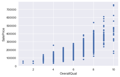
The most significant predictor of housing price is the OverallQuality of the property. Additionally, there is a nonlinear relation between this quality and SalePrice, with a quadratic term added to the model showing an even stronger correlation than the linear term.
I suggest a simplified model with six parameters to predict SalePrices. The linear model with ['LotArea', 'OverallQual', 'OverallCond', 'YearBuilt', 'GrLivArea', 'OverallQualSquared'] explains the variation in the data just about as well as the best model with twice as many parameters (difference in R-squared on a test set is less than 0.01). This parameter selection is stable over repeated selections of test and training data in a 2:1 split.
NAmes and CollgCr are the largest markets (with CollgCr also having high prices). NoRidge, NridgHt, and StoneBr have the highest average sale prices. Crawfor has prices that are trending higher.
Detailed Analysis
Read in the data
First save the list of variables we are allowed to use, and read in the just the training data from those columns.
avail_columns = ["LotArea", "Utilities", "Neighborhood", "BldgType", "HouseStyle", "OverallQual" \
           ,"OverallCond", "YearBuilt", "YearRemodAdd", "RoofStyle", "RoofMatl" \
           ,"GrLivArea", "FullBath", "HalfBath", "BedroomAbvGr", "KitchenAbvGr" \
           ,"MoSold", "YrSold", "SalePrice"]


df = pd.read_csv("train.csv", usecols=avail_columns)
print df
| LotArea | Utilities | Neighborhood | BldgType | HouseStyle | OverallQual | OverallCond | YearBuilt | YearRemodAdd | RoofStyle | RoofMatl | GrLivArea | FullBath | HalfBath | BedroomAbvGr | KitchenAbvGr | MoSold | YrSold | SalePrice | |
|---|---|---|---|---|---|---|---|---|---|---|---|---|---|---|---|---|---|---|---|
| 0 | 8450 | AllPub | CollgCr | 1Fam | 2Story | 7 | 5 | 2003 | 2003 | Gable | CompShg | 1710 | 2 | 1 | 3 | 1 | 2 | 2008 | 208500 |
| 1 | 9600 | AllPub | Veenker | 1Fam | 1Story | 6 | 8 | 1976 | 1976 | Gable | CompShg | 1262 | 2 | 0 | 3 | 1 | 5 | 2007 | 181500 |
| 2 | 11250 | AllPub | CollgCr | 1Fam | 2Story | 7 | 5 | 2001 | 2002 | Gable | CompShg | 1786 | 2 | 1 | 3 | 1 | 9 | 2008 | 223500 |
| 3 | 9550 | AllPub | Crawfor | 1Fam | 2Story | 7 | 5 | 1915 | 1970 | Gable | CompShg | 1717 | 1 | 0 | 3 | 1 | 2 | 2006 | 140000 |
| 4 | 14260 | AllPub | NoRidge | 1Fam | 2Story | 8 | 5 | 2000 | 2000 | Gable | CompShg | 2198 | 2 | 1 | 4 | 1 | 12 | 2008 | 250000 |
| 5 | 14115 | AllPub | Mitchel | 1Fam | 1.5Fin | 5 | 5 | 1993 | 1995 | Gable | CompShg | 1362 | 1 | 1 | 1 | 1 | 10 | 2009 | 143000 |
| 6 | 10084 | AllPub | Somerst | 1Fam | 1Story | 8 | 5 | 2004 | 2005 | Gable | CompShg | 1694 | 2 | 0 | 3 | 1 | 8 | 2007 | 307000 |
| 7 | 10382 | AllPub | NWAmes | 1Fam | 2Story | 7 | 6 | 1973 | 1973 | Gable | CompShg | 2090 | 2 | 1 | 3 | 1 | 11 | 2009 | 200000 |
| 8 | 6120 | AllPub | OldTown | 1Fam | 1.5Fin | 7 | 5 | 1931 | 1950 | Gable | CompShg | 1774 | 2 | 0 | 2 | 2 | 4 | 2008 | 129900 |
| 9 | 7420 | AllPub | BrkSide | 2fmCon | 1.5Unf | 5 | 6 | 1939 | 1950 | Gable | CompShg | 1077 | 1 | 0 | 2 | 2 | 1 | 2008 | 118000 |
| 10 | 11200 | AllPub | Sawyer | 1Fam | 1Story | 5 | 5 | 1965 | 1965 | Hip | CompShg | 1040 | 1 | 0 | 3 | 1 | 2 | 2008 | 129500 |
| 11 | 11924 | AllPub | NridgHt | 1Fam | 2Story | 9 | 5 | 2005 | 2006 | Hip | CompShg | 2324 | 3 | 0 | 4 | 1 | 7 | 2006 | 345000 |
| 12 | 12968 | AllPub | Sawyer | 1Fam | 1Story | 5 | 6 | 1962 | 1962 | Hip | CompShg | 912 | 1 | 0 | 2 | 1 | 9 | 2008 | 144000 |
| 13 | 10652 | AllPub | CollgCr | 1Fam | 1Story | 7 | 5 | 2006 | 2007 | Gable | CompShg | 1494 | 2 | 0 | 3 | 1 | 8 | 2007 | 279500 |
| 14 | 10920 | AllPub | NAmes | 1Fam | 1Story | 6 | 5 | 1960 | 1960 | Hip | CompShg | 1253 | 1 | 1 | 2 | 1 | 5 | 2008 | 157000 |
| 15 | 6120 | AllPub | BrkSide | 1Fam | 1.5Unf | 7 | 8 | 1929 | 2001 | Gable | CompShg | 854 | 1 | 0 | 2 | 1 | 7 | 2007 | 132000 |
| 16 | 11241 | AllPub | NAmes | 1Fam | 1Story | 6 | 7 | 1970 | 1970 | Gable | CompShg | 1004 | 1 | 0 | 2 | 1 | 3 | 2010 | 149000 |
| 17 | 10791 | AllPub | Sawyer | Duplex | 1Story | 4 | 5 | 1967 | 1967 | Gable | CompShg | 1296 | 2 | 0 | 2 | 2 | 10 | 2006 | 90000 |
| 18 | 13695 | AllPub | SawyerW | 1Fam | 1Story | 5 | 5 | 2004 | 2004 | Gable | CompShg | 1114 | 1 | 1 | 3 | 1 | 6 | 2008 | 159000 |
| 19 | 7560 | AllPub | NAmes | 1Fam | 1Story | 5 | 6 | 1958 | 1965 | Hip | CompShg | 1339 | 1 | 0 | 3 | 1 | 5 | 2009 | 139000 |
| 20 | 14215 | AllPub | NridgHt | 1Fam | 2Story | 8 | 5 | 2005 | 2006 | Gable | CompShg | 2376 | 3 | 1 | 4 | 1 | 11 | 2006 | 325300 |
| 21 | 7449 | AllPub | IDOTRR | 1Fam | 1.5Unf | 7 | 7 | 1930 | 1950 | Gable | CompShg | 1108 | 1 | 0 | 3 | 1 | 6 | 2007 | 139400 |
| 22 | 9742 | AllPub | CollgCr | 1Fam | 1Story | 8 | 5 | 2002 | 2002 | Hip | CompShg | 1795 | 2 | 0 | 3 | 1 | 9 | 2008 | 230000 |
| 23 | 4224 | AllPub | MeadowV | TwnhsE | 1Story | 5 | 7 | 1976 | 1976 | Gable | CompShg | 1060 | 1 | 0 | 3 | 1 | 6 | 2007 | 129900 |
| 24 | 8246 | AllPub | Sawyer | 1Fam | 1Story | 5 | 8 | 1968 | 2001 | Gable | CompShg | 1060 | 1 | 0 | 3 | 1 | 5 | 2010 | 154000 |
| 25 | 14230 | AllPub | NridgHt | 1Fam | 1Story | 8 | 5 | 2007 | 2007 | Gable | CompShg | 1600 | 2 | 0 | 3 | 1 | 7 | 2009 | 256300 |
| 26 | 7200 | AllPub | NAmes | 1Fam | 1Story | 5 | 7 | 1951 | 2000 | Gable | CompShg | 900 | 1 | 0 | 3 | 1 | 5 | 2010 | 134800 |
| 27 | 11478 | AllPub | NridgHt | 1Fam | 1Story | 8 | 5 | 2007 | 2008 | Gable | CompShg | 1704 | 2 | 0 | 3 | 1 | 5 | 2010 | 306000 |
| 28 | 16321 | AllPub | NAmes | 1Fam | 1Story | 5 | 6 | 1957 | 1997 | Gable | CompShg | 1600 | 1 | 0 | 2 | 1 | 12 | 2006 | 207500 |
| 29 | 6324 | AllPub | BrkSide | 1Fam | 1Story | 4 | 6 | 1927 | 1950 | Gable | CompShg | 520 | 1 | 0 | 1 | 1 | 5 | 2008 | 68500 |
| ... | ... | ... | ... | ... | ... | ... | ... | ... | ... | ... | ... | ... | ... | ... | ... | ... | ... | ... | ... |
| 1430 | 21930 | AllPub | Gilbert | 1Fam | 2Story | 5 | 5 | 2005 | 2005 | Gable | CompShg | 1838 | 2 | 1 | 4 | 1 | 7 | 2006 | 192140 |
| 1431 | 4928 | AllPub | NPkVill | TwnhsE | 1Story | 6 | 6 | 1976 | 1976 | Gable | CompShg | 958 | 2 | 0 | 2 | 1 | 10 | 2009 | 143750 |
| 1432 | 10800 | AllPub | OldTown | 1Fam | 1Story | 4 | 6 | 1927 | 2007 | Gable | CompShg | 968 | 2 | 0 | 4 | 1 | 8 | 2007 | 64500 |
| 1433 | 10261 | AllPub | Gilbert | 1Fam | 2Story | 6 | 5 | 2000 | 2000 | Gable | CompShg | 1792 | 2 | 1 | 3 | 1 | 5 | 2008 | 186500 |
| 1434 | 17400 | AllPub | Mitchel | 1Fam | 1Story | 5 | 5 | 1977 | 1977 | Gable | CompShg | 1126 | 2 | 0 | 3 | 1 | 5 | 2006 | 160000 |
| 1435 | 8400 | AllPub | NAmes | 1Fam | 1Story | 6 | 9 | 1962 | 2005 | Gable | CompShg | 1537 | 1 | 1 | 3 | 1 | 7 | 2008 | 174000 |
| 1436 | 9000 | AllPub | NAmes | 1Fam | 1Story | 4 | 6 | 1971 | 1971 | Gable | CompShg | 864 | 1 | 0 | 3 | 1 | 5 | 2007 | 120500 |
| 1437 | 12444 | AllPub | NridgHt | 1Fam | 1Story | 8 | 5 | 2008 | 2008 | Hip | CompShg | 1932 | 2 | 0 | 2 | 1 | 11 | 2008 | 394617 |
| 1438 | 7407 | AllPub | OldTown | 1Fam | 1Story | 6 | 7 | 1957 | 1996 | Gable | CompShg | 1236 | 1 | 0 | 2 | 1 | 4 | 2010 | 149700 |
| 1439 | 11584 | AllPub | NWAmes | 1Fam | SLvl | 7 | 6 | 1979 | 1979 | Hip | CompShg | 1725 | 2 | 1 | 3 | 1 | 11 | 2007 | 197000 |
| 1440 | 11526 | AllPub | Crawfor | 1Fam | 2.5Fin | 6 | 7 | 1922 | 1994 | Gable | CompShg | 2555 | 2 | 0 | 3 | 1 | 9 | 2008 | 191000 |
| 1441 | 4426 | AllPub | CollgCr | TwnhsE | 1Story | 6 | 5 | 2004 | 2004 | Gable | CompShg | 848 | 1 | 0 | 1 | 1 | 5 | 2008 | 149300 |
| 1442 | 11003 | AllPub | Somerst | 1Fam | 2Story | 10 | 5 | 2008 | 2008 | Gable | CompShg | 2007 | 2 | 1 | 3 | 1 | 4 | 2009 | 310000 |
| 1443 | 8854 | AllPub | BrkSide | 1Fam | 1.5Unf | 6 | 6 | 1916 | 1950 | Gable | CompShg | 952 | 1 | 0 | 2 | 1 | 5 | 2009 | 121000 |
| 1444 | 8500 | AllPub | CollgCr | 1Fam | 1Story | 7 | 5 | 2004 | 2004 | Gable | CompShg | 1422 | 2 | 0 | 3 | 1 | 11 | 2007 | 179600 |
| 1445 | 8400 | AllPub | Sawyer | 1Fam | SFoyer | 6 | 5 | 1966 | 1966 | Gable | CompShg | 913 | 1 | 0 | 3 | 1 | 5 | 2007 | 129000 |
| 1446 | 26142 | AllPub | Mitchel | 1Fam | 1Story | 5 | 7 | 1962 | 1962 | Gable | CompShg | 1188 | 1 | 0 | 3 | 1 | 4 | 2010 | 157900 |
| 1447 | 10000 | AllPub | CollgCr | 1Fam | 2Story | 8 | 5 | 1995 | 1996 | Gable | CompShg | 2090 | 2 | 1 | 3 | 1 | 12 | 2007 | 240000 |
| 1448 | 11767 | AllPub | Edwards | 1Fam | 2Story | 4 | 7 | 1910 | 2000 | Gable | CompShg | 1346 | 1 | 1 | 2 | 1 | 5 | 2007 | 112000 |
| 1449 | 1533 | AllPub | MeadowV | Twnhs | SFoyer | 5 | 7 | 1970 | 1970 | Gable | CompShg | 630 | 1 | 0 | 1 | 1 | 8 | 2006 | 92000 |
| 1450 | 9000 | AllPub | NAmes | Duplex | 2Story | 5 | 5 | 1974 | 1974 | Gable | CompShg | 1792 | 2 | 2 | 4 | 2 | 9 | 2009 | 136000 |
| 1451 | 9262 | AllPub | Somerst | 1Fam | 1Story | 8 | 5 | 2008 | 2009 | Gable | CompShg | 1578 | 2 | 0 | 3 | 1 | 5 | 2009 | 287090 |
| 1452 | 3675 | AllPub | Edwards | TwnhsE | SLvl | 5 | 5 | 2005 | 2005 | Gable | CompShg | 1072 | 1 | 0 | 2 | 1 | 5 | 2006 | 145000 |
| 1453 | 17217 | AllPub | Mitchel | 1Fam | 1Story | 5 | 5 | 2006 | 2006 | Gable | CompShg | 1140 | 1 | 0 | 3 | 1 | 7 | 2006 | 84500 |
| 1454 | 7500 | AllPub | Somerst | 1Fam | 1Story | 7 | 5 | 2004 | 2005 | Gable | CompShg | 1221 | 2 | 0 | 2 | 1 | 10 | 2009 | 185000 |
| 1455 | 7917 | AllPub | Gilbert | 1Fam | 2Story | 6 | 5 | 1999 | 2000 | Gable | CompShg | 1647 | 2 | 1 | 3 | 1 | 8 | 2007 | 175000 |
| 1456 | 13175 | AllPub | NWAmes | 1Fam | 1Story | 6 | 6 | 1978 | 1988 | Gable | CompShg | 2073 | 2 | 0 | 3 | 1 | 2 | 2010 | 210000 |
| 1457 | 9042 | AllPub | Crawfor | 1Fam | 2Story | 7 | 9 | 1941 | 2006 | Gable | CompShg | 2340 | 2 | 0 | 4 | 1 | 5 | 2010 | 266500 |
| 1458 | 9717 | AllPub | NAmes | 1Fam | 1Story | 5 | 6 | 1950 | 1996 | Hip | CompShg | 1078 | 1 | 0 | 2 | 1 | 4 | 2010 | 142125 |
| 1459 | 9937 | AllPub | Edwards | 1Fam | 1Story | 5 | 6 | 1965 | 1965 | Gable | CompShg | 1256 | 1 | 1 | 3 | 1 | 6 | 2008 | 147500 |
1460 rows × 19 columns
Explore each variable and correlations
Check the info on the data frame for column data types and null values. Any column with dtype of int64 is complete since a single string or NaN entry would change the dtype for the entire column. The object columns are all expected to have string values, so no worries there. Check the value_counts on the object columns for mis-spelled labels.
df['YrSold'].describe()
count    1460.000000
mean     2007.815753
std         1.328095
min      2006.000000
25%      2007.000000
50%      2008.000000
75%      2009.000000
max      2010.000000
Name: YrSold, dtype: float64
df.BldgType.value_counts()
1Fam      1220
TwnhsE     114
Duplex      52
Twnhs       43
2fmCon      31
Name: BldgType, dtype: int64
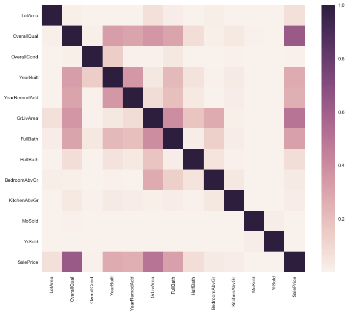
Need to decide which variables should become dummified. We do this with categorical classifications that we expect to have a strong impact on the result. Utilities and RoofMatl may not be good choices since there is so little variation… though we should inspect them to see if there is a strong correlation with the price.
correl = df.corr()**2
fig, ax = plt.subplots(figsize=(12,10))
sns.heatmap(correl);
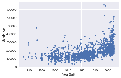
for i in avail_columns:
if df[i].dtype == int:
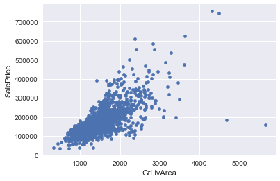
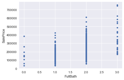
df.plot(x=i,y="SalePrice",kind="scatter")
plt.show()
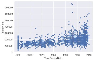
Explore nonlinear relationships
Some of the features are correlated in a nonlinear fashion with the sales price, so I will check correlations with the logarithm of the sales price, and with the logarithm of the features… I can also try polynomial fits with the features. Overall Quality, YearBuilt,
Looks like some features show outliers (such as LotArea being greather than 60000 units, HalfBath ==2, or BedroomAbvGr > 5, KitchenAbvGr == 0 or 3). One can make a stron case that the estimate for these lots should be given by a different function than for the others… Perhaps these are times when the categorical variables would work well?
plt.scatter(df.OverallQual**2,df.SalePrice)
#df.corr()
<matplotlib.collections.PathCollection at 0x1178f5750>
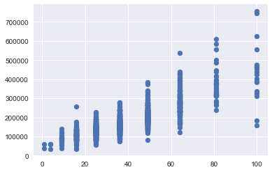
df["OverallQualSquared"] = df.OverallQual**2
df["YearBuiltSquared"] = df.YearBuilt**2
Training test split
features = ['LotArea', 'OverallQual', 'OverallCond', 'YearBuilt', 'YearRemodAdd',
       'GrLivArea', 'FullBath', 'HalfBath',
       'BedroomAbvGr', 'KitchenAbvGr', 'MoSold', 'YrSold',
       'OverallQualSquared', 'YearBuiltSquared']

X = df[features]
y = df['SalePrice']

X_train, X_test, y_train, y_test = train_test_split(X, y, test_size=.33)
Fitting
# REGRESSION MODELS

results = []
for n in range(1,len(features)+1):
    max_r2 = 0
    best_features = []
    for cols in itertools.combinations(features, n):
        fit_xtrain = X_train[list(cols)]
        fit_xtest = X_test[list(cols)]

#FIT LINEAR MODEL
        line = lm.LinearRegression(normalize=True)

#for algorithm in [line, lasso, ridge]:
        for algorithm in [line]:
            ## Fit model to data
            model = algorithm.fit(fit_xtrain,y_train)

            test_r2 = algorithm.score(fit_xtest, y_test)
#             print "Test r2 score : {}".format(test_r2);
            if test_r2 > max_r2:
                max_r2 = test_r2
                coeff_sum = abs(algorithm.coef_).mean()
                mse = mean_squared_error(y_true=y_test, y_pred=algorithm.predict(fit_xtest))
                best_features = list(cols)
    results.append( (max_r2,coeff_sum, mse, best_features))
results
[(0.64493256596024184,  3738.6815185367077,  2186715449.1880145,
  ['OverallQualSquared']),
 (0.72915774869635741,  1444.2671637627586,  1668006914.8561254,
  ['GrLivArea', 'OverallQualSquared']),
 (0.75483471919634171,   939.9441940699586,  1509872930.4412842,
  ['YearBuilt', 'GrLivArea', 'OverallQualSquared']),
 (0.79589913657403477,  12011.917742913709,  1256973939.1988173,
  ['LotArea',       'OverallQual',       'OverallCond',
   'YearBuilt',       'GrLivArea',       'HalfBath',
   'KitchenAbvGr',       'OverallQualSquared']),
 (0.79640356966477699,  10782.082461790924,  1253867341.6152034,
  ['LotArea',       'OverallQual',       'OverallCond',
   'YearBuilt',       'GrLivArea',       'HalfBath',
   'BedroomAbvGr',       'KitchenAbvGr',       'OverallQualSquared']),
 (0.79670268601380689,  9925.112054464651,  1252025206.0690444,
  ['LotArea',       'OverallQual',       'OverallCond',
   'YearBuilt',       'GrLivArea',       'FullBath',
   'HalfBath',       'BedroomAbvGr',       'KitchenAbvGr',
   'OverallQualSquared']),
 (0.79624488667288296,  7607.3176169180288,  1254844605.4153514,
  ['LotArea',       'OverallQual',       'OverallCond',
   'YearBuilt',       'YearRemodAdd',       'GrLivArea',
   'FullBath',       'HalfBath',       'BedroomAbvGr',
   'KitchenAbvGr',       'MoSold',       'YrSold',
   'OverallQualSquared',       'YearBuiltSquared'])]
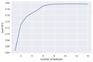
Plot the progression of the best coefficient of determination as the number of features selected grows.
plt.plot(range(1,len(results)+1),[r[0] for r in results])
plt.xlabel("number of features")
plt.ylabel("best R^2")
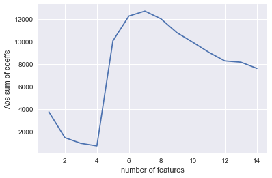
Plot the absolute sum of the coefficients. Note that this only works when the features are normalized in some fashion before fitting. A significant increase in this sum is an indication of the model being overfit. Comparing this to the difference in R2 score would make a good cross check for overfitting.
plt.plot(range(1,len(results)+1),[r[1] for r in results])
plt.xlabel("number of features")
plt.ylabel("Abs sum of coeffs")
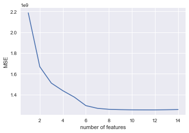
Plot the best mean squared error (MSE) for each number of features corresponding to the best R2 score.
plt.plot(range(1,len(results)+1),[r[2] for r in results])
plt.xlabel("number of features")
plt.ylabel("MSE")
Compare the be R2 score with a value from near the point of diminishing R2 returns.
print max([r[0] for r in results])
results[5]
0.796794359218


(0.79010957401318027,     12257.811452486383,     1292629492.7138808,
 ['LotArea',      'OverallQual',      'OverallCond',
  'YearBuilt',      'GrLivArea',      'OverallQualSquared'])
Selected model
The r-squared value for the test set drops plateaus around 0.83, when six features are used. The set selected is: [‘LotArea’, ‘OverallQual’, ‘OverallCond’, ‘YearBuilt’, ‘GrLivArea’, ‘OverallQualSquared’]. The linear model with these features selected from the entire training set will capture most of the trends in the data without risking overfitting or storing extraneous data (particualrly since one of the features selected is derived from another!).
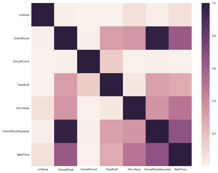
The model with 13 parameters (excluding only month sold) consistently beats the model with 6 parameters, but only by a small margin. Considering the colinearity between many of the parameters (seen in the heatmap during initial data exploration) a smaller parameter set is desireable. Selecting parameters with Ridge and Lasso was not as successful as the fitting with limited parameter sets, so I have opted for the latter.
A model with 8 parameters sometimes did slightly better than the model with 6, but the feature selection was not consistent (due to colinearity), so I went for the six final parameters. The differences in R^2 between the full model and 6 parameters were someitmes as large as 0.01, while the 8 parameter fit was half that. This increase in success did not seem to justify the loss in certainty over the best feature set.
correl = df[['LotArea', 'OverallQual', 'OverallCond', 'YearBuilt', 'GrLivArea', 'OverallQualSquared','SalePrice']].corr()**2
fig, ax = plt.subplots(figsize=(12,10))
sns.heatmap(correl);
Neighborhood summary
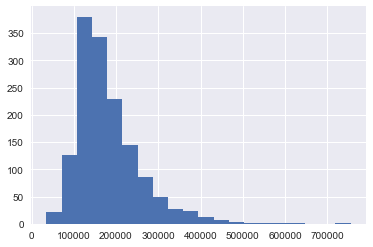
The first figure shows the distribution of sales prices. Anything over $170k will be toward the high end of the market. Anything over $300k is really an exclusive property.
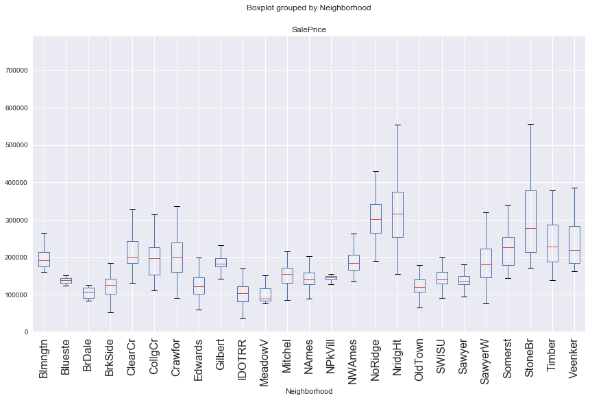
Below that is a box plot graph showing the distribution of prices in each neighborhood. It seems NoRidge, NridgHt, and StoneBr have higher median SalePrice than the other neighborhoods. A t test on this hypothesis shows significance with a p-value less than 0.0001.
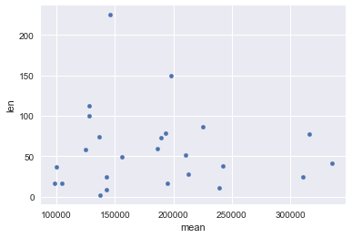
Below that are tables showing the number of homes sold and the mean sale price in each neighborhood. Interestingly, there is no correlation between those two variables (as seen by the scatter plot below the tables.
NridgHt, in particular, has a good combination of sale price and sale volume. NAmes and CollgCr are two other neighborhoods that have lower home prices, but much more sales volume. CollgCr is a good market with over 100 homes sold in the dataset, and a mean sale price of nearly $200k.
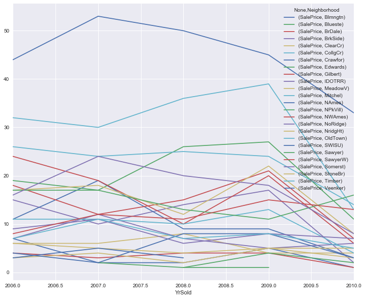
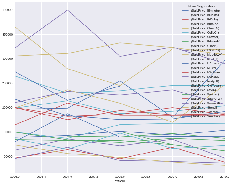
Finally, I have some charts and tables showing how sale price and volume change over time in each neighborhood in the data set. This is a fairly stable market in terms of meaningful rankings of the neighborhoods. Crawfor, however, is worth watching, as it’s mean sale price has been trending upward during the duration of the data set.
To sum up: NAmes and CollgCr are the largest markets (with CollgCr also having high prices). NoRidge, NridgHt, and StoneBr have the highest average sale prices. Crawfor has prices that are trending higher.
df.SalePrice.hist(bins=20)
<matplotlib.axes._subplots.AxesSubplot at 0x1178356d0>
df.boxplot(column="SalePrice", by="Neighborhood",figsize=(14,8),rot=90,fontsize=16)
<matplotlib.axes._subplots.AxesSubplot at 0x1182aa550>
mask = (df['Neighborhood'] =='NoRidge' ) \
        | (df['Neighborhood']=='NridgHt') \
        | (df['Neighborhood']=='StoneBr')
tstat, pval = stats.ttest_ind(a= df[mask]['SalePrice'], \
                b= df[[not x for x in mask]]['SalePrice'], \
                equal_var=False)
print 2* pval
6.94365699791e-37
df.pivot_table(index=["Neighborhood"], values=["SalePrice"], \
               aggfunc=[np.mean,len]).sort_values(('mean','SalePrice'),ascending=False)
| mean | len | |
|---|---|---|
| SalePrice | SalePrice | |
| Neighborhood | ||
| NoRidge | 335295 | 41 |
| NridgHt | 316270 | 77 |
| StoneBr | 310499 | 25 |
| Timber | 242247 | 38 |
| Veenker | 238772 | 11 |
| Somerst | 225379 | 86 |
| ClearCr | 212565 | 28 |
| Crawfor | 210624 | 51 |
| CollgCr | 197965 | 150 |
| Blmngtn | 194870 | 17 |
| Gilbert | 192854 | 79 |
| NWAmes | 189050 | 73 |
| SawyerW | 186555 | 59 |
| Mitchel | 156270 | 49 |
| NAmes | 145847 | 225 |
| NPkVill | 142694 | 9 |
| SWISU | 142591 | 25 |
| Blueste | 137500 | 2 |
| Sawyer | 136793 | 74 |
| OldTown | 128225 | 113 |
| Edwards | 128219 | 100 |
| BrkSide | 124834 | 58 |
| BrDale | 104493 | 16 |
| IDOTRR | 100123 | 37 |
| MeadowV | 98576 | 17 |
df.pivot_table(index=["Neighborhood"], values=["SalePrice"], \
               aggfunc=[np.mean,len]).sort_values(('len','SalePrice'),ascending=False)
| mean | len | |
|---|---|---|
| SalePrice | SalePrice | |
| Neighborhood | ||
| NAmes | 145847 | 225 |
| CollgCr | 197965 | 150 |
| OldTown | 128225 | 113 |
| Edwards | 128219 | 100 |
| Somerst | 225379 | 86 |
| Gilbert | 192854 | 79 |
| NridgHt | 316270 | 77 |
| Sawyer | 136793 | 74 |
| NWAmes | 189050 | 73 |
| SawyerW | 186555 | 59 |
| BrkSide | 124834 | 58 |
| Crawfor | 210624 | 51 |
| Mitchel | 156270 | 49 |
| NoRidge | 335295 | 41 |
| Timber | 242247 | 38 |
| IDOTRR | 100123 | 37 |
| ClearCr | 212565 | 28 |
| StoneBr | 310499 | 25 |
| SWISU | 142591 | 25 |
| Blmngtn | 194870 | 17 |
| MeadowV | 98576 | 17 |
| BrDale | 104493 | 16 |
| Veenker | 238772 | 11 |
| NPkVill | 142694 | 9 |
| Blueste | 137500 | 2 |
df.pivot_table(index=["Neighborhood"], values=["SalePrice"], \
               aggfunc=[np.mean,len]).plot.scatter(x="mean",y="len")
<matplotlib.axes._subplots.AxesSubplot at 0x118173610>
df.pivot_table(index=["YrSold"], values=["SalePrice"], \
               columns=["Neighborhood"],aggfunc=np.mean \
              ).plot(figsize=(12,10))
<matplotlib.axes._subplots.AxesSubplot at 0x117bace50>
df.pivot_table(index=["Neighborhood"], values=["SalePrice"], \
               columns=["YrSold"],aggfunc=np.mean \
              ).sort_values(("SalePrice",2010),ascending=False)
| SalePrice | |||||
|---|---|---|---|---|---|
| YrSold | 2006 | 2007 | 2008 | 2009 | 2010 |
| Neighborhood | |||||
| StoneBr | 365046.0 | 279585.0 | 245000.0 | 319967.0 | 318886.0 |
| NridgHt | 305491.0 | 310833.0 | 332422.0 | 323143.0 | 308281.0 |
| Crawfor | 196635.0 | 198777.0 | 254411.0 | 180211.0 | 296833.0 |
| NoRidge | 322333.0 | 399730.0 | 304750.0 | 323875.0 | 289938.0 |
| ClearCr | 199166.0 | 236333.0 | 208991.0 | 169875.0 | 246850.0 |
| Timber | 264485.0 | 229470.0 | 234361.0 | 245437.0 | 245160.0 |
| Somerst | 210268.0 | 233248.0 | 225631.0 | 236315.0 | 206762.0 |
| CollgCr | 199016.0 | 213999.0 | 187718.0 | 192317.0 | 203700.0 |
| Blmngtn | 217087.0 | 183350.0 | 175447.0 | 176720.0 | 192000.0 |
| NWAmes | 199463.0 | 175267.0 | 193820.0 | 185133.0 | 187428.0 |
| Gilbert | 200250.0 | 181967.0 | 186000.0 | 199955.0 | 185500.0 |
| SawyerW | 164787.0 | 209300.0 | 184080.0 | 183934.0 | 184076.0 |
| Mitchel | 150036.0 | 136731.0 | 165280.0 | 167860.0 | 166950.0 |
| NAmes | 138985.0 | 142962.0 | 151553.0 | 143880.0 | 153665.0 |
| SWISU | 130125.0 | 187500.0 | 139612.0 | 141048.0 | 141333.0 |
| NPkVill | NaN | 141500.0 | 140000.0 | 146937.0 | 136750.0 |
| Sawyer | 149735.0 | 133935.0 | 128900.0 | 136925.0 | 132400.0 |
| OldTown | 135963.0 | 114794.0 | 147670.0 | 116378.0 | 122464.0 |
| Edwards | 134403.0 | 132588.0 | 132473.0 | 123855.0 | 111445.0 |
| BrkSide | 112746.0 | 135737.0 | 121707.0 | 134994.0 | 96500.0 |
| BrDale | 96750.0 | 113833.0 | 95225.0 | 118625.0 | 88000.0 |
| IDOTRR | 95758.0 | 118933.0 | 91642.0 | 89580.0 | 86278.0 |
| MeadowV | 123466.0 | 105850.0 | 98000.0 | 88400.0 | 81333.0 |
| Blueste | NaN | NaN | 151000.0 | 124000.0 | NaN |
| Veenker | 273333.0 | 214900.0 | 244000.0 | NaN | NaN |
df.pivot_table(index=["YrSold"], values=["SalePrice"], columns=["Neighborhood"],aggfunc=len \
              ).plot(figsize=(12,10))
<matplotlib.axes._subplots.AxesSubplot at 0x117da6f90>